
The thief’s lockpick slides into the lock with caution, but the pervasive stench and discomfort disrupt his concentration. He feels the lock resisting, but he doesn’t give up. Then he hears a sound that he doesn’t like. When he withdraws his lockpick, he realizes that half of it is stuck in the door, which diminishes their chances of escape to nothing.
The jailer, in his haste to see what was happening, reaches the door and opens the metal peephole, but he is immediately hit by an unbearable stench. He realizes too late that he has covered his feet with the noxious substance that had spread in the cell. Taken aback, the jailer lets out a disgusted cry and starts cursing the prisoners.
Jailer: (furious) By the hells, what is this?! You filthy bunch!
Despite his discomfort, the jailer takes a look inside the cell and realizes that the prisoners have caused significant damage. He tries to open the door but finds that the keys won’t fit the lock. They’ve blocked the cell. A smug smile crosses his face.
Jailer: (satisfied) By the gods, they’ve blocked the door! How did they do that?! Stay in your mess, you idiots!
The adventurers, still prisoners, now find themselves trapped in their own filth. Escape seems impossible, despite the persistent stench of the cell. The magician, however, continues her exposition on the triangular probability law undisturbed, attempting to find meaning in this chaotic situation.
The Law of Two Dice
Magician: My dear friends, now that you have a solid understanding of the discrete uniform law, let me talk to you about another intriguing distribution, the triangular law, which manifests when we roll two six-sided dice and sum the values obtained on their top faces.
Unlike the uniform distribution we discussed earlier, the triangular law features a different distribution of probabilities.
For a simple roll of a balanced and unbiased six-sided die, the probability of obtaining any value from 1 to 6 is evenly distributed, that is, 1/6 for each outcome. This constitutes a discrete uniform law. However, when we roll two dice and add their values, the outcomes are no longer uniformly distributed but instead follow a triangular distribution.

Sum of the dice is 2: Probability 1/36
Sum of the dice is 3: Probability 2/36
Sum of the dice is 4: Probability 3/36
Sum of the dice is 5: Probability 4/36
Sum of the dice is 6: Probability 5/36
Sum of the dice is 7: Probability 6/36
Sum of the dice is 8: Probability 5/36
Sum of the dice is 9: Probability 4/36
Sum of the dice is 10: Probability 3/36
Sum of the dice is 11: Probability 2/36
Sum of the dice is 12: Probability 1/36
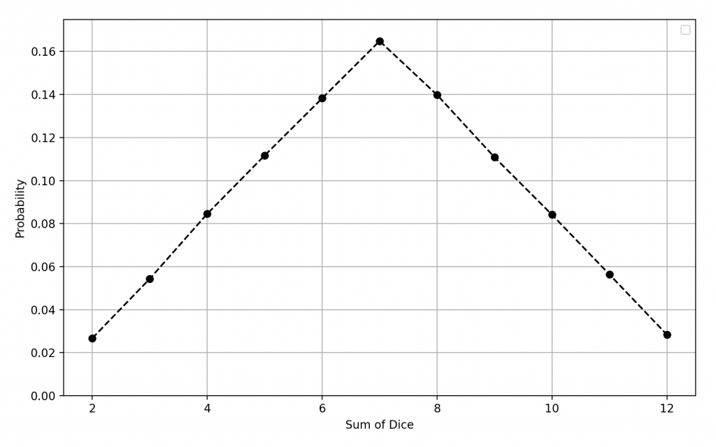
As you can see, the most probable sum is 7, with a probability of 6/36, while the extremes, 2 and 12, have the lowest probability, with only 1/36.
There are various possible combinations with two six-sided dice to achieve a specific sum. Let me list them:
To get a sum of 2, there is only one possible combination: 1+1.
To get a sum of 3, there are two possible combinations: 1+2 and 2+1.
To get a sum of 4, there are three possible combinations: 1+3, 2+2, and 3+1.
And so on, until we reach a sum of 12, which has only one possible combination: 6+6.
This triangular distribution is fascinating because it reflects how probabilities are distributed when combining the results of two dice. Keep in mind that this knowledge may prove useful in your future adventures as it allows you to estimate the chances of success when dealing with situations that involve complex dice rolls.
It's not Over !
However, it’s essential to remember that everything that has just been narrated is not the true end of the story but rather a variation of what could have happened.
In the world of role-playing games, possibilities are endless, and the fate of our adventurers often depends on the players’ choices and the Game Master’s decisions. So, let the quest continue because each adventure is unique and unpredictable, and new challenges await our brave heroes in the darkest corners.
Find the real ending.
Bibliography
M. Fréchet, M. Halbwachs, Le calcul des probabilités à la portée de tous, Dunod, 1924, 297 p.
C. Barboianu, Probability Guide to Gambling. The Mathematics of Dice, Slots, Roulette, Baccarat, Blackjack, Poker, Lottery and Sport Bets, INFAROM Publishing, 2006, 316 p
P. Nahin, Digital Dice. Computational Solutions to Practical Probability Problems, Princeton University Press, 2008, 263 p.
I. Stewart, Do Dice Play God?: The Mathematics of Uncertainty, 2019
import matplotlib.pyplot as plt
import numpy as np

# Number of simulations
n_simulations = 100000

# Simulations of rolling two dice and calculating sums
results = np.random.randint(1, 7, size=(n_simulations, 2))
sums = np.sum(results, axis=1)

# Calculation of probability density
unique, counts = np.unique(sums, return_counts=True)
probability = counts / n_simulations

# Creating the probability density plot
plt.figure(figsize=(10, 6))
plt.plot(unique, probability, marker='o', linestyle='--', color='black')

# Labeling axes and adding a title
plt.xlabel('Sum of Dice')
plt.ylabel('Probability')

# Limiting the y-axis scale from 0 to the maximum probability
plt.ylim(0, max(probability) + 0.01)

# Displaying the legend
plt.legend()

# Displaying the plot
plt.grid(True)
plt.show()