
Rogue: (whispering) I have a bad feeling about that lever. We don’t know what it might trigger.
Ranger: (cautious) You’re right; caution is in order in this situation. Let’s not pull that lever without more information.
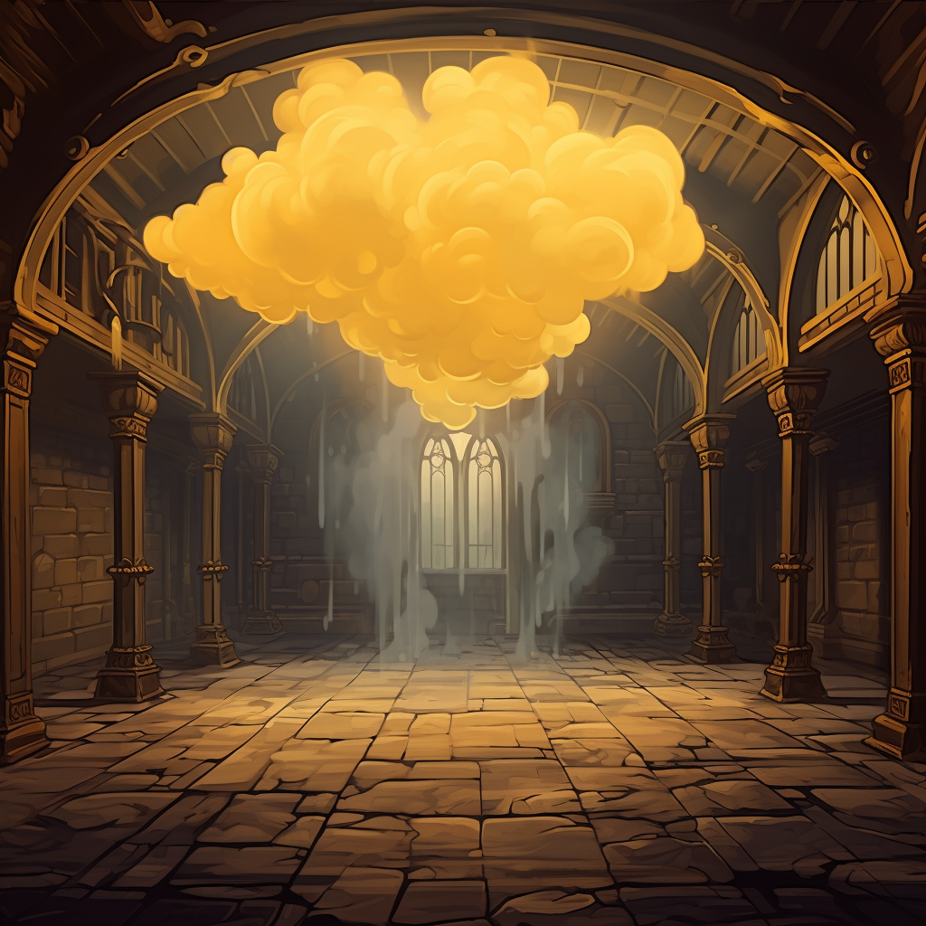
So, they decide not to touch the lever for now, opting not to risk an unpredictable reaction. However, at that very moment, time seems to freeze around them, and the luminous entity in the glass cage begins to speak.
Azar: (with an ethereal voice) You’ve shown wisdom by avoiding the lever, but time is of the essence. A team of soldiers approaches, led by a powerful mage. To overcome these foes, you’ll need to understand the intricacies of the multinomial probability distribution.
The Law of Coins
He explained that the binomial distribution is based on n independent binary choices, much like flipping a coin n times, where the two possible outcomes are Heads or Tails (n being any number such as 1, 12, 100, etc.). In the case of a fair coin, the probability of Heads, denoted as \(p_1\) was 0.5, while the probability of Tails, denoted as \(p_2\) (or \(1-p_1\)), was also 0.5. Furthermore, he pointed out that if the coin were biased, these probabilities (\(p_1\) and \(p_2\)) could take other values, such as 0.4 or 0.6, revealing an imbalance (see the article Toss a Coin to Your Witcher).
In mathematical terms, the binomial distribution is a discrete probability distribution described by two parameters: the number of trials n (or the number of experiments conducted) and the probability of success \(p_1\) (it could also be \(p_2\)).
Azar continued his presentation by introducing the formula for calculating the probability of getting exactly \(n_1\) Tail and \(n_2\) Head Tails in a series of n trials. It looked like this:
\begin{equation*}\mathbb{P}(N_1 = n_1, N_2 = n_2) =\frac{n!}{n_1!n_2!} \cdot p_1^{n_1} \cdot p_2^{n_2}\end{equation*}
where n! represents the multiplication of all integers from 1 to n, so \(n!= n\times (n-1)\times\cdots\times 3\times 2\times 1\), for example \(4!=4\times 3\times 2\times 1= 24\). Of course, this formula might not be the most common one taught in mathematics classes, but we won’t delve into that here.
However, he added that this distribution did not account for the order in which the results occurred (order does not matter).
To illustrate his teaching, he called upon the group’s leader, the ranger, who agreed to flip a coin five times in a row. The adventurers, their eyes fixed on the suspended coin, watched with fascination as the final sequence revealed: TTHTH.
With his mystical aura, he explained that the probability of getting precisely this sequence was \(\frac{1}{2^{5}}\), which meant there was a one in 32 chance of this sequence occurring. The adventurers were beginning to grasp the importance of probability calculations in situations like this.
Azar emphasized that the binomial distribution accounted for all possible ways to get three Heads out of the five flips (which is 20 possibilities), and he reminded them of the corresponding formula.
\begin{equation*}\mathbb{P}(N_1 = 3, N_2=2) =\frac{5!}{3!2!} \cdot p_1^3 \cdot p_2^{2} = 20 \times \frac{1}{2^{5}}\end{equation*}

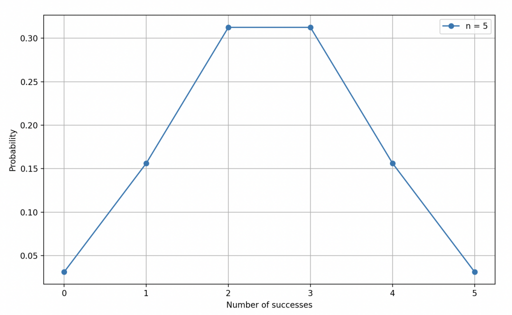
Binomial law of parameters \(n=5\) and \(p_1=0.5\).
He then explained that the binomial distribution had several key characteristics essential for understanding and analyzing a given experiment.
The expectation of the binomial distribution, denoted by \(\mathbb{E}(N_1)\), was defined as the expected value of the number of successes in n trials, based on the probability \(p_1\) of success in an individual trial:
\begin{equation*}\mathbb{E}(N_1) = n \cdot p_1 = 0.5\times n\end{equation*}
Azar added that the variance of the binomial distribution was calculated as follows, quantifying the spread of results around the expectation and providing insight into the stability or variability of the outcomes:
\begin{equation*}V(N_1) = n \cdot p_1 \cdot p_2 = 0.25\times n\end{equation*}
Azar then enlightened the adventurers about the mode of the binomial distribution, explaining that the mode was the value of \(n_1\) that maximized the probability. For a balanced coin, he emphasized that the mode was located at \(\frac{n}{2}\), meaning that the most likely outcome was to get an equal number of Heads and Tails.
He also mentioned the skewness and kurtosis of the binomial distribution, acknowledging that the calculations could be more complex than the previous ones.
Skewness, denoted by \(\gamma_1(N_1)\), was defined as a measure of the asymmetry of the binomial distribution, with the following formula:
\begin{equation*}\gamma_1(N_1) = \frac{p_2-p_1}{\sqrt{np_1p_2}}=0\end{equation*}
Clearly, when the coin is balanced, we obtain a symmetrical curve with respect to the mean.
As for kurtosis, symbolized by\(\gamma_2(N_1)\), it assessed the shape of the distribution compared to a standard normal distribution (bell-shaped curve), with the following formula:
\begin{equation*}\gamma_2(N_1) = \frac{1-6p_1p_2}{np_1p_2}\end{equation*}
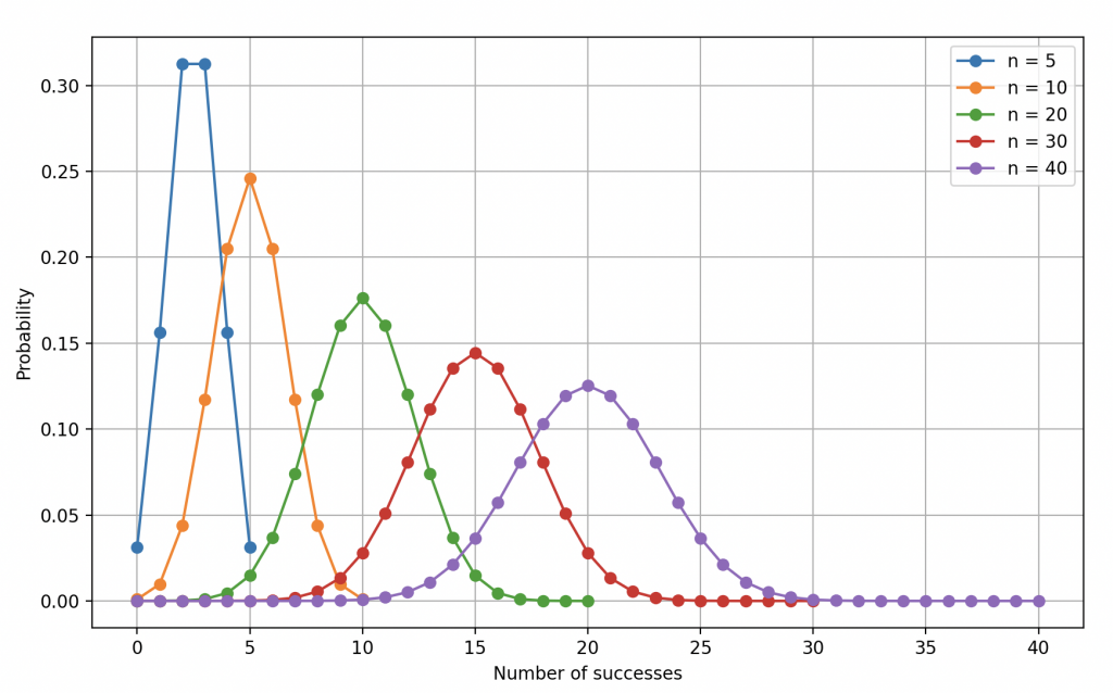
Binomial law of parameters \(n=5,10,20,30,40\) and \(p_1=0.5\).
The Law of Dice
The dreaded moment was approaching. Four soldiers, staunch defenders of their garrison, advanced to confront our brave heroes. To triumph over these formidable opponents, they would need to harness the power of their magical dice and make good rolls.
Soldier 1: 3 times the number 6, 1 time the number 5, 0 times the number 4, 1 time the number 3, 1 time the number 2, and 1 time the number 1.
Soldier 2: 0 times the number 6, 1 time the number 5, 3 times the number 4, 0 times the number 3, 1 time the number 2, and 2 times the number 1.
Soldier 3: 2 times the number 6, 1 time the number 5, 1 time the number 4, 1 time the number 3, 1 time the number 2, and 1 time the number 1.
Soldier 4: 1 time the number 6, 1 time the number 5, 1 time the number 4, 1 time the number 3, 3 times the number 2, and 0 times the number 1.
Mage: 7 times the number 6, 0 times the number 5, 0 times the number 4, 0 times the number 3, 0 times the number 2, and 0 times the number 1.
In this situation, the complexity arose from the fact that instead of having only two possible outcomes, as in a simple coin toss, they now had six possible results, and this could vary depending on circumstances, sometimes more, sometimes fewer (depending on the dice you use).
Azar: (in a soothing voice) To help you better understand, let’s focus on a standard six-sided die. Since the dice are not loaded, the probability of rolling a 6, which we’ll denote as \(p_6\), is the same as rolling a 1 (and all the others), denoted as \(p_1\) and they are each 1/6. Thus, it’s like a fair coin toss, where each outcome has an equal chance of occurring (the discrete uniform distribution).
Azar went on to explain that, by analogy with the binomial distribution, for any die, the probability of getting \(n_6\) values of 6, \(\cdots\), \(n_1\) values of 1 in n rolls of a die is:
\begin{equation*}
\mathbb{P}(N_6=n_6, \cdots, N_1=n_1) =\frac{n!}{n_6!n_5!n_4!n_3!n_2!n_1!} \cdot p_1^{n_1} \cdot p_2^{n_2}\cdot p_3^{n_3}\cdot p_4^{n_4}\cdot p_5^{n_5}\cdot p_6^{n_6}
\end{equation*}
and for a fair die, this simplifies to:
\begin{equation*}
\mathbb{P}(N_6=n_6, \cdots, N_1=n_1) =\frac{n!}{n_6!n_5!n_4!n_3!n_2!n_1!} \cdot\left(\frac{1}{6}\right)^n
\end{equation*}
This formula took into account the number of ways to arrange the die outcomes for each roll and the probabilities of getting each face. In the case of a fair die, this formula was simplified using the 1/6 probability for each face.
Azar then applied these mathematical concepts to explain that the probability of defeating Soldier 1 was very low, calculated at around 0.003. Our heroes remained perplexed, realizing that their chances of success were slim.
\begin{equation*}\mathbb{P}(N_6=3, N_5 = 1, N_4 = 0, N_3 = 1, N_2 = 1, N_1=1)=\frac{7!}{3!1!0!1!1!1!}\cdot\left( \frac{1}{6}\right)^7\approx0,003\end{equation*}
Facing their destiny, the adventurers rolled the dice, hoping to obtain the magical sequence. Incredibly, they managed to defeat the first soldier by rolling the sequence 1, 6, 6, 6, 5, 2, 3, a combination that had an extremely low chance of occurring, only 1 in 279,936, like all possible configurations in 7 rolls.
Azar did not delve into the properties of such a distribution much, only the most classical ones, the expected value and the variance, which have the same formulations as for the binomial distribution. He also did not teach about its graphical representation, as humanity cannot easily visualize curves in more than three dimensions. Here, there are 6! Thus, it was only necessary to adapt to the representation of the binomial distribution and use a little imagination.
Our heroes had triumphed over the first obstacle, but the road ahead of them remained long and uncertain. They had now grasped the crucial importance of probability and the multinomial distribution in their quest. Armed with this powerful knowledge, they prepared to face the remaining soldiers with unwavering determination and a glimmer of hope in their eyes. The battle was far from won, but they were ready to confront the uncertainty that awaited them.
However, despite their mastery of probabilities, our adventurers were not invincible. Their journey eventually led them to the mage, whose odds of defeat were even slimmer. Fate decreed it so, and our heroes were defeated by the mage, despite their bravery.
Deception !
As our heroes were swept away by the mysteries of their destiny, Azar revealed a profound truth to them: the order of events had no fundamental importance, unlike the series of improbable coincidences that had led them to him (he advised them to calculate the probability of reaching him without dying). These fortuitous circumstances had unexpectedly shaped their destiny, as if the narrative thread had woven itself with the threads of chance.
It was as if this entire journey had been a game, a game that had started when the thief had flipped that coin to the dwarf in the tavern. Every roll of the dice in the cell, every roll against the soldiers, everything had contributed to sculpting their destiny, leading them inexorably to Azar. Reality and fiction had intertwined, creating an exciting adventure where probability had become the guiding thread.
Our heroes, in a blend of amusement and reflection, recalled the lessons of probability, realizing how much understanding such concepts could influence the course of their story. They savored their return, aware that even in the narrative of their lives, chance had its own place, weaving a complex and captivating tapestry.
Bibliography
P. Bogaert, Probabilités pour scientifiques et ingénieurs : Introduction au calcul des probabilités, De Boeck Supérieur, 2005, 402 p
E. Gossett, Discrete Mathematics with Proof, Hoboken (N.J.), John Wiley & Sons, 2009, 904 p
E. Lesigne, Heads or tails : an introduction to limit theorems in probability, Providence (R.I.), AMS, 2005, 150 p.
D. Foata, A. Fuchs et J. Ranchi, Calcul des probabilités : Cours, exercices et problèmes corrigés, Paris/Berlin/Heidelberg etc., Dunod, 2012, 3e éd., 368 p.
import matplotlib.pyplot as plt
import scipy.stats as stats

# Parameters of the binomial distribution
p = 0.5  # Probability of success
n_values = [5, 10, 20, 30, 40]  # Different values of n

# Create the graph
plt.figure(figsize=(10, 6))

# Simulation and plotting of curves for each value of n
for n in n_values:
    x = range(n + 1)
    y = [stats.binom.pmf(k, n, p) for k in x]
    plt.plot(x, y, marker='o', label=f'n = {n}')

# Labeling of axes and adding a title
plt.xlabel('Number of successes')
plt.ylabel('Probability')

# Display the legend
plt.legend()

# Display the graph
plt.grid(True)
plt.show()