
The Monte Carlo Method
The Monte Carlo method is an efficient mathematical strategy that is applied to approximate results that are otherwise intractable to calculate with precision. It relies on the use of pseudo-random numbers to simulate random events and derive probabilistic outcomes. A simple illustration to grasp this method would be to envision an army of stormtroopers randomly firing upon a target. By virtue of the Monte Carlo method, we can estimate the stormtroopers’ precision rate by simulating their random shooting and counting the number of shots that strike the target. But especially they can estimate areas.
Tis method is grounded on the law of large numbers, which asserts that if a large number of independent random experiments are conducted, the frequency of the outcomes will converge towards the theoretical probability. For example, if you toss a balanced coin a very large number of times, it will appear tail or head half the time. To employ this method, one must first define a simulation space of random events, generate pseudo-random numbers to mimic these events, and tally the number of occurrences that transpire within a specific region of interest. This information is then used to estimate the probability of a particular event.
For instance, to estimate the precision rate of the stormtroopers, we could define a simulation space that represents the target, let them shoot, and count the number of shots that strike the target. By using the ratio of the number of shots that strike the target to the total number of shots, we can estimate the precision rate of the stormtroopers. To do so,
- Put one stormtrooper in the closed and huge shooting range.
- Let’s draw a circle of radius 25 meters in the center of the squared back wall of 50 meters.
- Now, it’s time to order to the stormtrooper to fire.
“Stormtrooper, attention, target in the back wall in sight, fire one thousand shot.”
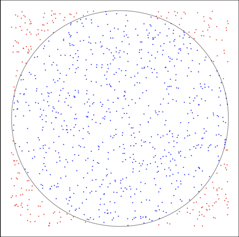
Figure 1: A stormtrooper trying to shot the target and the result obtained with one thousand shots.
According to the target, we have the proof that he is not really good at shooting. In fact, he shoots uniformly in the back wall, i.e., in mathematical terms, it means that the probability of striking a defined zone in the back wall is the same as striking another one with the same area. This probability is called continuous uniform distribution. These non-skills will be used to estimate the value of mathematical constants (such as π) and a lot more things.
Estimation of π and the Millennium Falcon’s Area
Before continuing, let’s recall that the area of a square of side R is (S_{square}=R²) and the area of a circle of radius R is (S_{circle}=π R²). We will start with the simplest estimation: that of π. This works by using the same steps as outlined previously
- Put the army of one million and identical stormtroopers in the closed and huge shooting range.
- Draw a circle of radius 25 meters within the squared back wall of 50 meters.
- Recall the order.
“Stormtroopers, attention, target in the back wall in sight, fire one shot.”
- Count the number of impacts (or points) that fall inside the circle.
- Use the proportion of impacts inside the circle to the total number of impacts generated to estimate π. Specifically, you can use the following formula:
Repeat steps several times or increase your army to get a more precise estimate of π.
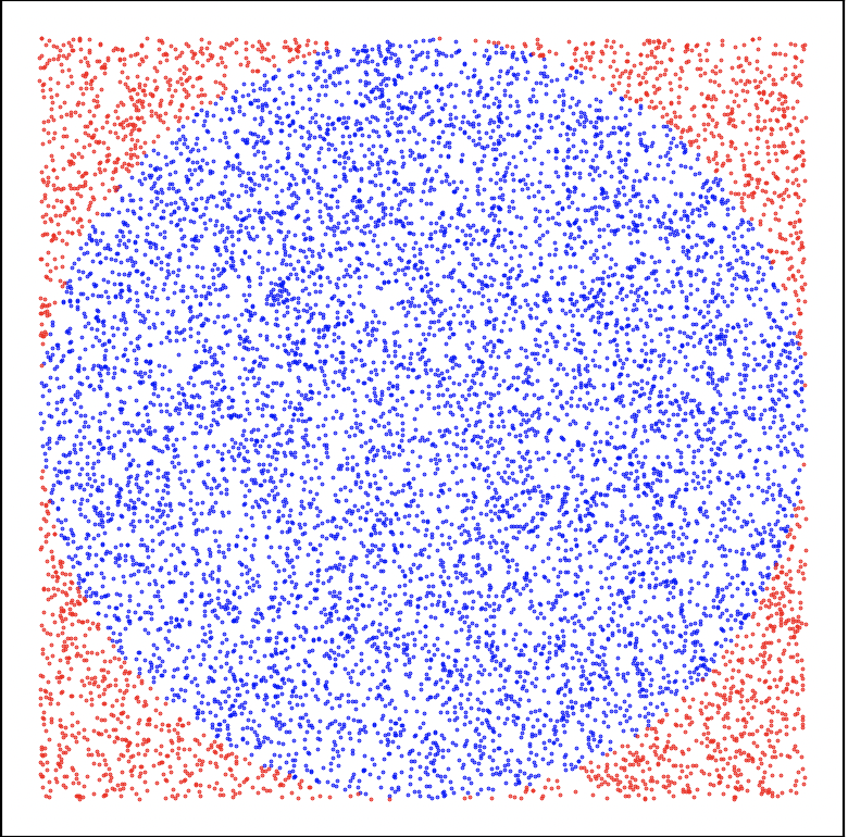
Figure 2: The army has arrived and launch first 10 thousands shots.
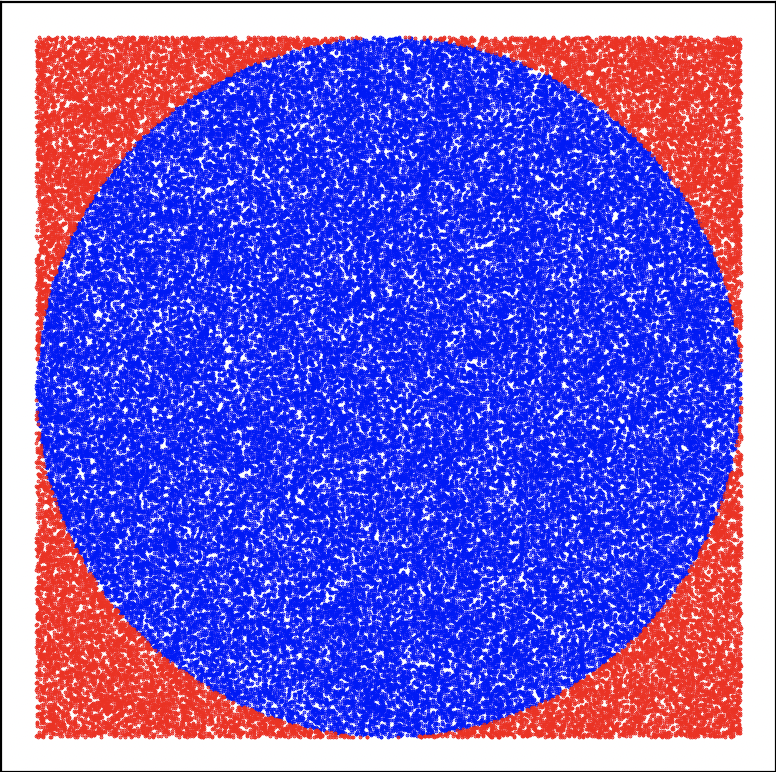
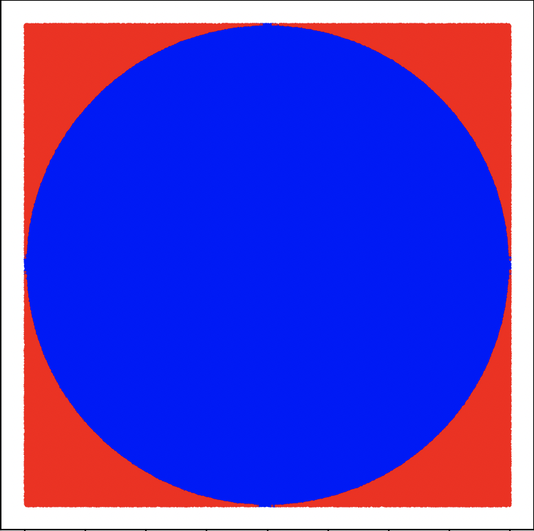
Figure 3: From left to right, 100 thousands and 1 million shots.
Similarly, one can use this method to estimate the area of the Millennium Falcon, a famous spaceship from the Star Wars series that measures 35 meters in length and 25 meters in width.
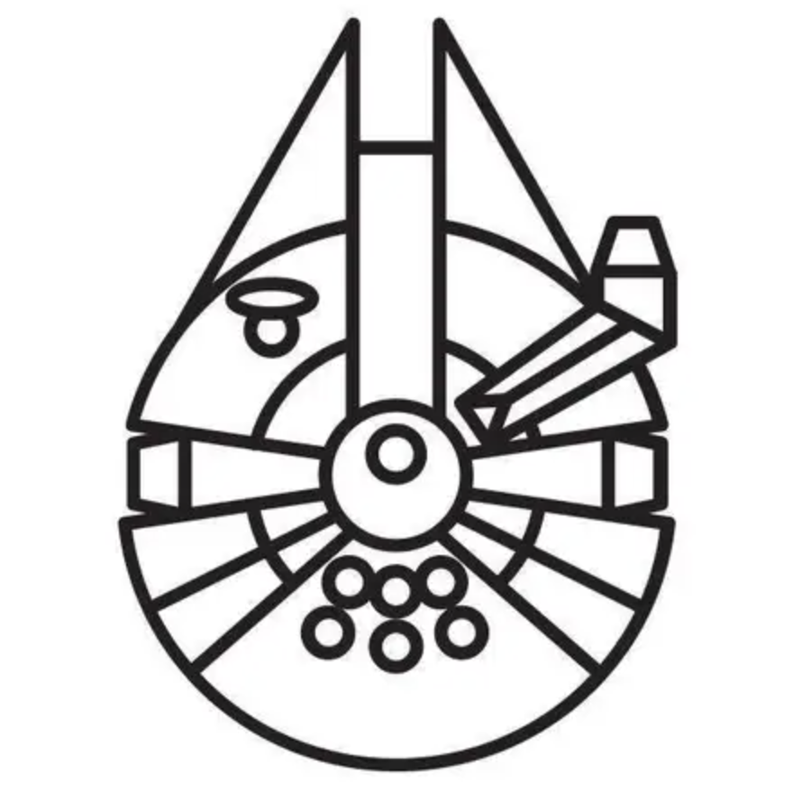
Figure 4: Here is the real spaceship photo and plan.
The methodology will almost be the same. We use a computer simulation where stormtroopers randomly shoot at the surface of the spaceship. Each point where a “stormtrooper” hits the surface is recorded and the total area is then calculated by counting the total number of points and comparing it to the total size of the spaceship’s surface. This method is very effective because it takes into account the irregular shapes of the spaceship’s surface, which could make it difficult for a more traditional area estimation. But, unfortunately, this will lead to the total destruction of the spaceship!
- Put the army of stormtroopers in a closed and huge shooting range.
- Draw a 35m x 25m rectangle to represent the surface of the back wall and stick the millennium falcon on it.
- Order the stormtroopers to fire.
- Count the number of shots that strike the surface of the Millennium Falcon.
- Use the proportion of shots that strike the surface of the Millennium Falcon to the total number of shots to estimate the area of the Millennium Falcon. Specifically, you can use the following formula:
- Repeat steps several times or increase the number of stormtroopers to get a more precise estimate of the area of the Millennium Falcon.
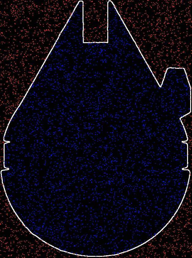
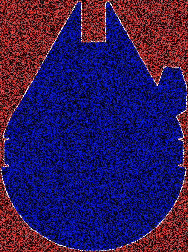

Figure 5: From left to right, with 10 thousands, 100 thousands and 1 million shots.
The accuracy of the Monte Carlo method for estimating areas depends on the number of randomly generated shots. The more impacts you generate, the more accurate your estimate will be. However, it is important to note that even if you generate a large number of impacts, you will never be able to calculate the exact value of the area you consider. For example, with 1 million stormtroopers, you can get an estimate of π with an accuracy of about 2 decimal places. For the millenium falcon area, we get approximately 400.855m².
The importance of lack of precision
The Monte Carlo method relies heavily on the generation of random numbers to simulate random events. This is where the lack of precision of the stormtroopers comes in. In the previous example, the stormtroopers’ lack of precision in shooting represents the randomness required for the Monte Carlo method to work effectively (here, they shoot perfectly bad). Without this randomness, the method would not be able to accurately approximate results.
Let me explain this concept by introducing Han Solo, a highly skilled marksman, into the simulation. The distribution of shots fired would no longer be uniformly random, but rather, it would be weighted towards the areas where Han Solo aims. More precisely, if we estimate its precision rate as we did with the stormtroopers, we observe that he shoots almost perfectly well.

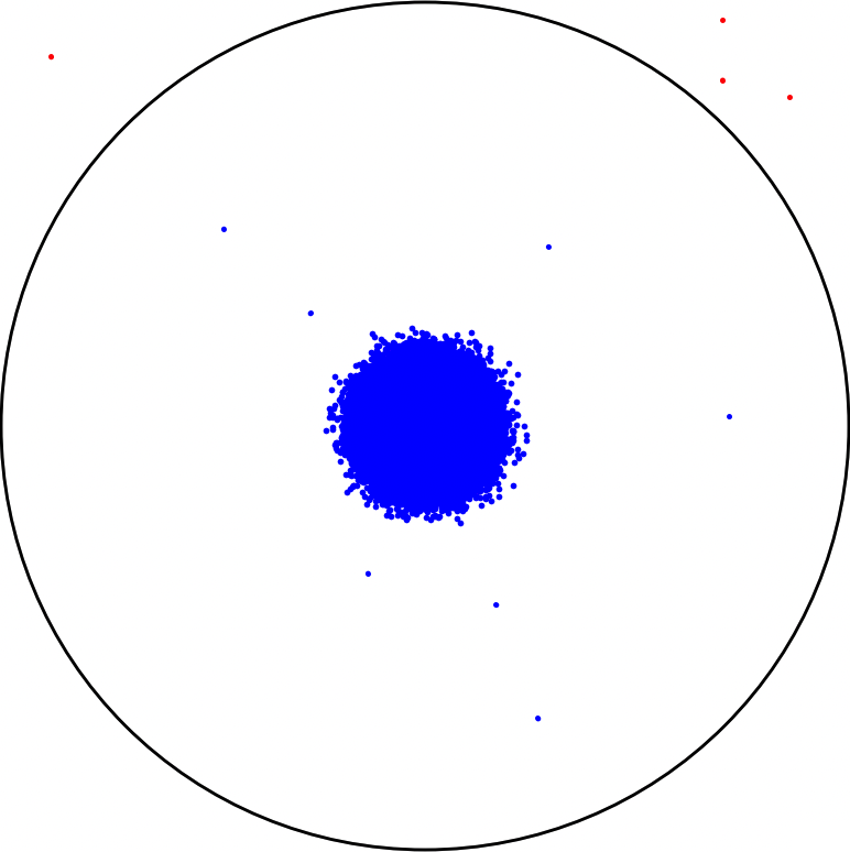
Figure 6: Han solo firing one million shots.
Maybe because Chewbacca is bothering him or because he has dust in his eye, and this is why its precision rate is not 100 percent (he says). Now, how good is he at estimating π? By using the same formula
it seems that π is more or less equal to 4 with 1 million of shots.
This highlights an important consideration when using the Monte Carlo method - the accuracy of the results depends heavily on the random nature of the simulation. Introducing biases or non-uniform distributions can greatly impact the effectiveness of the method. Roughly speaking, it means that to be accurate, the random numbers generated must be truly random and not follow a predictable pattern or being precise.
Generation of random numbers
Generating random numbers is a fundamental task in many fields, ranging from computer science to cryptography and simulations. While we often think of randomness as something that occurs naturally, such as the roll of a die or the flip of a coin, many random numbers used in computing are actually generated through sophisticated algorithms or physical phenomena.
One widely used method is the pseudo-random number generator, which produces a sequence of numbers that appears random, but is actually calculated deterministically from an initial “seed” value. Although not truly random, pseudo-random generators are highly efficient and unpredictable enough to meet most practical needs. However, they are subject to periodicities and correlations in the sequences produced, which can pose security risks in certain applications. By using the Star Wars analogy, it consists in taking a perfect imperial sniper which follows a shooting pattern; you only have to order the first target to hit and each shoot will be a defined function of the previous one.
Figure 7: An imperial sniper with a part of his shooting pattern.
Now, imagine that you are a rebel spy and you want to send a secret message to your base. For this, you need a random number that will serve as an encryption key. You could use a pseudorandom number generator to create one, but there is always a risk that the Empire has been able to predict the sequence of numbers you are going to use. To make sure that your encryption key is truly random, you could use a quantum number generator.
In this example, the pseudorandom number generator would be like an Empire soldier who follows a predefined and easily predictable attack plan as the imperial sniper. On the other hand, the quantum number generator would be like a scientist rebel who exploits the unique properties of light sabers to find unpredictable solutions to each situation. As quantum numbers are generated from unpredictable quantum phenomena such as polarization, phase, or frequency of photons, the Empire cannot predict the sequence of numbers you will use, making your secret message much safer. These generators produce numbers that are truly random and impossible to replicate. While still relatively new and expensive, quantum random number generators hold great promise for applications requiring the highest levels of security and unpredictability.
The Versatility and Power of the Monte Carlo Method
To sum up, the Monte Carlo method is a versatile and powerful mathematical technique that allows for the approximation of complex results that are otherwise difficult to calculate precisely. The use of random or pseudo-random numbers to simulate random events and determine probabilistic outcomes makes it an effective tool for various applications, as demonstrated by the simulations of stormtroopers’ shootings. The method’s applications extend beyond estimating mathematical constants and areas of irregular shapes, to include predicting the outcome of elections, simulating population growth, and estimating the probability of rolling a certain number on a dice game.
The Monte Carlo method is a valuable tool for numerous fields, such as physics, engineering, and finance, making it an essential component of the mathematician and statistician’s toolkit.
Bibliography
M. Kalos, P. Whitlock, Monte Carlo Methods, 2008.
D. P. Kroese, T. Taimre, Z.I. Botev, Handbook of Monte Carlo Methods, 2011.
D. P. Kroese, T. Brereton, T. Taimre, Z.I. Botev, Why the Monte Carlo method is so important today, 2014.
S. Weinzierl, Introduction to Monte Carlo methods, 2000.
Code appendix
Estimation of π by Stormtroopers
import random

def estimate_pi(n):
    num_inside = 0
    for _ in range(n):
        x = random.uniform(-1, 1)
        y = random.uniform(-1, 1)
        if x**2 + y**2 <= 1:
            num_inside += 1
    return 4 * num_inside / n

print(f"π ≈ {estimate_pi(1_000_000):.4f}")
Estimation of the Millennium Falcon’s area
import cv2, numpy as np, random

img = cv2.imread("falcon2.png", cv2.IMREAD_GRAYSCALE)
_, thresh = cv2.threshold(img, 127, 255, cv2.THRESH_BINARY_INV)
contours, _ = cv2.findContours(thresh, cv2.RETR_EXTERNAL, cv2.CHAIN_APPROX_SIMPLE)
h, w = img.shape[:2]

n = 1_000_000
hits = sum(
    1 for _ in range(n)
    if cv2.pointPolygonTest(contours[0],
        (random.randint(0, w-1), random.randint(0, h-1)), False) >= 0
)
area = (hits / n) * 35 * 25  # real dimensions in metres
print(f"Estimated area: {area:.2f} m²")
Estimation of π by Han Solo (Gaussian shooting)
import random, math

num_shots = 1_000_000
circle_hits = 0
for _ in range(num_shots):
    x = random.gauss(0, 0.05)
    y = random.gauss(0, 0.05)
    if math.sqrt(x**2 + y**2) <= 1:
        circle_hits += 1

print(f"π ≈ {4 * circle_hits / num_shots:.4f}")