Toss a Coin to Your Witcher
By Jordan Moles on July 25, 2023
Credit: Netflix
In the heart of the mysterious lands of The Witcher universe, where swords clash and spells unleash, a valuable lesson emerges from the depths of probability and destiny. Inspired by a chance encounter in the mists of a casino bar, this lesson invites us to delve into the intricacies of the law of large numbers, while the player’s ruin looms like a threatening shadow. Prepare to be transported into an enchanting narrative, where dice are cast, and games of chance play their captivating symphony.
The Stranger and the Challenge of Destiny
On a tumultuous evening, a solitary witcher named Geralt of Rivia roams the dark streets of a city in search of respite. The echoes of laughter and enchanting melodies guide him to a mysterious bar, the Casino of Destiny. Driven by an irresistible curiosity, he crosses the ornate doors and enters a world where fate is sealed by a simple roll of the dice. Among the lively crowd in the bar, the witcher is drawn to an enigmatic stranger. With a mischievous twinkle in his eye, the stranger takes out a sparkling coin from his satchel. His sly smile betrays a clear intention: he wants to challenge the witcher to a little table game. Intrigued, Geralt accepts the invitation, preparing to face destiny itself.
Credit: Netflix
The stranger, with an enigmatic voice, lays out the rules of the game. Both of them will wager their respective fortunes in the game, assuming Geralt and the stranger both start with 1000 gold coins. In each round, destiny oscillates between the players, thus determining their fortune on a coin toss. Each victory grants a gain of 1, while each defeat comes with an equivalent loss. This bewitching dance continues until one of the players is irreversibly ruined, condemned to face the consequences of their choices.
Let us now translate this situation into probabilistic terms, where “destiny” is represented by a probability p, a value between 0 and 1. A sequence of independent and identically distributed random variables, symbolized by \(X_i\) where i is the i-th round, plays a crucial role in the course of the game. Each variable \(X_i\) takes the value 1 with a probability p, indicating a victory, and the value -1 with a probability 1-p, indicating a defeat. Mathematically, this is denoted as follows:
\begin{align*}
\mathbb{P}(X_i=1)=p,\quad \mathbb{P}(X_i=-1)=1-p.
\end{align*}
We also note the Witcher’s fortune in round n, which is equal to the sum of his initial fortune and the results of his gains and losses in each round:
\begin{align*}
F_n = 1000 + \sum_{i=1}^n X_i.
\end{align*}
Simultaneously, the fortune of his opponent, intimately linked to his own, evolves through similar mechanisms, but with a fortune in each round of 2000-\(F_n\).
Probabilities Veiled: Geralt’s Quest Against Rigged Gambling
The rules of this game are deceitful, and Geralt senses that something is amiss. He suspects the old man of trying to cheat him. Immersed in an enigmatic situation, Geralt finds himself facing a captivating coin game. The possible outcomes are simple: Heads or Tails, with an equal probability of 50/50 if the coin is fair. However, he also knows that the coin could be biased, which worries him, with probabilities taking different values, such as 0, \(1/\pi\), or 1/100. The mystery deepens as the true probability remains unknown.
To unravel this mystery, Geralt mobilizes all his skills and available resources, even if it means losing money. He focuses on the first six coin tosses, which resulted in Heads, Tails, Heads, Tails, Tails, Tails (HTHTTT). At first glance, these results seem to indicate an imbalance. However, Geralt undertakes a thorough analysis of the probabilities associated with each possible configuration. He recalls that an old friend, Jacques Bernoulli, had presented him with a similar challenge. It was theoretically a random experiment with two possible outcomes, success or failure, each with a certain probability—exactly what he is facing now.
Jacques had told him that if the coin were fair, the probability of getting Heads first is 1/2, just like getting Tails first. By examining the different possible combinations (HT, HH, TT, TH), he realizes that the probability of getting Heads followed by Tails is 1/4, just like for the other combinations. This is because there are four equiprobable possibilities with a fair coin. Geralt remembers the reasoning well and becomes aware of the importance of details in this quest. He also realizes that, for three tosses, there are eight possible configurations. Among these, there is one chance in eight of getting Heads, Tails, Heads (HTH). Geralt quickly understand the extent of the calculations involved in this analysis. The more tosses there are, the lower the probability of obtaining a specific configuration becomes. For example, the probability of getting the configuration Heads, Tails, Heads, Tails, Tails, Tails (HTHTTT) is \(1/2^6\), a relatively low probability.
However, Geralt’s goal is not limited to determining specific configurations. His true interest lies in the proportion of Heads and Tails present in each configuration. In these terms, the sorcerer understands that he is facing a succession of n independent unbiased Bernoulli trials, where the random variable \(S_n\), which counts the number of successes, follows a binomial distribution. The probability of having k “Heads” in the sum is given by:
\begin{equation*}
\mathbb{P}(S_n=k)=\binom{n}{k}\frac{1}{2^n}.
\end{equation*}
We recall the following equality
$$\binom{n}{k}=\frac{n\times(n-1)\times\cdots\times 2\times 1}{(k\times(k-1)\times\cdots\times 2\times 1)(n-k)\times(n-k-1)\times \cdots\times 2\times 1}.$$
He anticipates that if the coin is tossed a very large number of times, the frequency of Heads or Tails will be revealed with great precision. His intuition proves correct, and mathematicians call this the “law of large numbers.”
In summary, the law of large numbers states that a fair coin, tossed an infinite number of times, will yield Heads and Tails with an equivalent frequency. Similarly, if the coin is biased, the Witcher will observe a proportion of Heads or Tails different from 50/50.
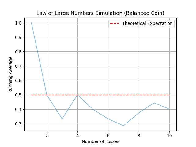
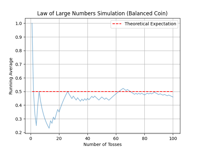


Simulation of coin tosses. The figures illustrate how the average of Heads tends to approach the theoretical expectation as the number of coin tosses increases (10, 100, 1000, 10000, and 100000), even with a biased coin. Thus, we can clearly observe that starting from 10000 tosses, the blue curve almost coincides with the theoretical average.
Geralt is aware of this mathematical truth, but he also knows that infinity is far too distant to reach, especially in the context of the game proposed by the stranger, where he could end up ruined very quickly.
The Power of Concentration: The Witcher Unravels the Mystery of the Biased Coin
In the game proposed by the stranger, Geralt doesn’t have the luxury of tossing the coin an infinite number of times to verify the frequency of the results. He realizes that he must harness his powers of concentration to the maximum to unravel the mystery of the biased coin. In search of an additional advantage, he decides to drink a potion of concentration, which stimulates his mind and clarity of vision.

Credit: Netflix

Credit: Netflix
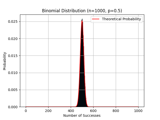
Histogram representing the frequency of Heads appearing in 1000 coin tosses, along with its bell-shaped theoretical curve.
To experimentally measure this frequency of occurrence, Geralt knows that he must count the number of Heads (+1) in the n coin tosses, divide it by the total number of tosses, and estimate the probability of deviation by a certain percentage u from the value of \(\frac{1}{2}\). This can be written using the previous formula, for all deviations u:
\begin{equation}\label{Gauss2}
\mathbb{P}\left(\left|\frac{S_n}{n}-\frac{1}{2}\right| > u\right) \leq 2e^{-2nu^2}.
\end{equation}
If his estimation exceeds the value on the right-hand side, then he is facing a biased coin. Thus, Geralt has a simple way to detect any potential bias in the coin.
Suddenly, time seems to freeze. The Witcher enters a deep trance that allows him to mentally toss the coin and perform all the necessary calculations using the previous formula.

Credit: Netflix

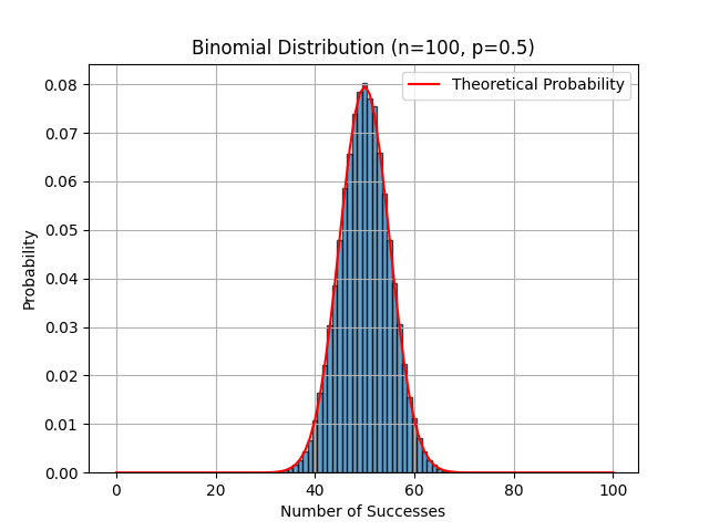
Histogram representing the frequency of Heads appearing in 10 coin tosses, along with its theoretical bell-shaped curve.
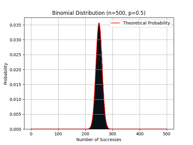
Histogram representing the frequency of Heads appearing in 100 and 500 coin tosses, along with their theoretical bell-shaped curves.
The approximate results of these calculations are presented in the following table and heatmap:
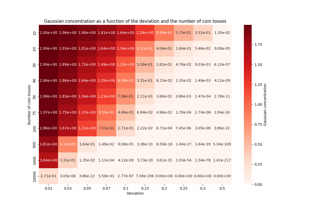
The table presents the results obtained by Geralt during his calculations for different numbers of coin tosses. The values in the cells correspond to the estimated probabilities that the frequency of Heads differs from \(\frac{1}{2}\) by a certain percentage (the deviation) based on the number of tosses.
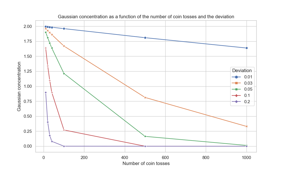
This graph represents the evolution of Gaussian concentration as a function of the deviation and the number of coin tosses.
By observing the data in the table and the evolution of the curves in the graph, we can draw the following conclusions:
• As the number of coin tosses increases, the probabilities of deviation decrease. This means that the more Geralt tosses coins, the more accurately he can estimate whether the coin is biased or not.
• For a small number of tosses (10 or 20), the probabilities of deviation remain relatively high. For example, for 10 tosses, the probability of a \(20\%\) deviation is 0.89, indicating a considerable possibility of bias. However, for 20 tosses, this probability decreases to 0.40, suggesting a reduction in uncertainty.
• As the number of tosses increases further (30, 40, 100, 500, 1000), the probabilities of deviation decrease drastically. For example, for 1000 tosses, the probability of a \(20\%\) deviation is extremely low, on the order of \(3.6 \times 10^{-35}\), indicating a high level of confidence that the coin is fair.
In summary, the table demonstrates that the more coin tosses Geralt performs, the more he can refine his estimation of the frequency of Heads and determine with greater certainty whether the coin is biased or not. The probabilities of deviation decrease rapidly as the number of tosses increases, which enhances the reliability of Geralt’s method to detect biased coins.
Thanks to his potion of concentration and his knowledge of probabilistic principles, the Witcher, Geralt, adjusts his game strategy and fully engages in the game proposed by the stranger. He tosses the provided coin 500 times and obtains a sequence of results where the number of Heads observed is 286, approximately \(7\%\) more than the expected number. Here is the sequence:
\begin{align*}
&0 0 1 0 1 0 0 0 0 1 1 1 1 1 0 1 0 1 0 0 0 1 0 11 0 1 0 1 0 0 1 0 1 1 1 1111111100011 1 1 0 0 1 1 1 1 1 1 0 1 1 0 1 0 0 1 0 1 \\
&1111 1 1 0 0 1 0 1 1 0 0 1 1 0 0 0 1 0 0 1 0 1 1 10 0 1 0 1 0 1 0 1 0 1 1 0 1 1 1 1 0 1 1 1 1 1 10 0 1 0 10 0 0 1 1 1 0 01 1 0 0 1\\
&1 1 0 0 1 0 1 1 1 1 1 0 0 1 0 1 0 1 0 1 1 1 1 11 1 1 1 0 0 1 1 1 0 0 0 1 0 1 1 0 1 1 0 0 1 1 0 0 0 1 0 1 1 1 1 10 0 0 0 11 1 1 0 0 1 0 \\
& 0 1 1 1 0 1 1 0 10 1 1 0 0 0 1 1 0 0 1 1 0 1 1 0 0 0 0 0 0 1 1 10 0 1 1 1 0 1 1 111 1 1 1 1 0 1 0 0 1 0 1 0 10 1 0 1 0 1 1 0 1 1 10 \\
& 1 1 0 0 0 1 1 1 0 1 0 00 1 1 1 1 0 1 0 0 0 0 1 1 1 0 0 1 1 1 1 0 1 0 11 0 0 1 0 1 0 1 0 1 0 0 1 0 1 0 1 1 0 1 0 0 0 01 0 1 10 1 0 0 1 \\
& 0 1 0 1 1 0 1 1 1 1 0 1 1 1 0 0 1 1 1111111 1 0 1 0 0 0 1 1 1 0 1 0 1 1 1 1 0 0 1 0 0 1 1 1 1 0 1 0 1 0 1 0 1 0 0 1 0 01 0 1 0 1 1 \\
&1 0 1 1 1 0 1 1 1 1 1 0 1 1 1 1 0 1 0 1 1 1111 0 1 1 0 0 1 1 1 0 0 1 1 1 0 1 0 1 0 0 1 0 0 0 1 1 0 1 0 1 0 0 0 1 1 0 00 0 1 1 10 1 0 \\
& 0 0 1 0 0 0 0 0 1 1 0 0 0 0 1 1 0
\end{align*}
By applying these calculations, Geralt estimates that the probability of obtaining such a deviation is approximately 0.01 (which is very low). He realizes that he is facing a scam and requests to restart the game using another coin, as the provided one is biased.
He turns to a casino dealer to obtain an official and fair coin, to continue the game in a just and fair manner.
Credit: Netflix
The Power of Concentration: The Plot of the Gambler’s Ruin: The Probability of Losing Everything
The game is now fair, and each player has an equal chance of winning. The Witcher is interested in the probability that the stranger goes broke before him, meaning that the stranger’s final fortune \(F_{\text{Stranger}}\) reaches 0 before 2000. Mathematically, this probability is expressed as:
\begin{align*}
\mathbb{P}_{Stranger}(1000)=\mathbb{P}_{1000}\left(F\text{ reaches } 0 \text{ before } 2000\right).
\end{align*}
This can also be rephrased using what is called stopping times. Stopping times are random times that can be determined from the information available on the process up to that point. Their value indicates the moment when a certain condition is satisfied or a certain quantity is reached. The stopping time may depend on past realizations of the process, but it cannot depend on the future. In our case, this could be the time (which we called round in our case) denoted as \(T_0\) when the stranger’s fortune reaches 0, or the time \(T_{2000}\) when it reaches 2000. In other words, it is the smallest time n at which \(F_n\) becomes zero or reaches 2000:
\begin{align*}
T_0=\inf\{n\geq 0,\quad F_n =0\}\quad \text{ and } \quad T_{2000}=\inf\{n\geq 0,\quad F_n =2000\}.
\end{align*}
It is evident that the longer the game is played, the more likely it is to come to an end, meaning that one of the two players goes broke. Thus, we can express the probability that the stranger loses all his gold before the witcher as the probability that the stopping time \(T_0\) is smaller than \(T_{2000}\):
\begin{align*}
\mathbb{P}_{Stranger}(1000)=\mathbb{P}_{1000}\left(T_0<T_{2000}\right).
\end{align*}
Also, it is important to note that the stranger’s fortune can take on all possible “states” (meaning his fortune can be any number between 0 and 2000). Let’s denote this value as k. Thus, the probability that, starting with a fortune of value k, he reaches 0 before 2000 is:
\begin{align*}
\mathbb{P}_{Stranger}(k)=\mathbb{P}_{k}\left(T_0<T_{2000}\right).
\end{align*}
This probability depends only on the value of the fortune in the previous round. Indeed, since only one gold coin is played in each round, each player can either win or lose only one coin and not, for example, 4 coins at once. Without going into specific details and keeping it general, this means that the previous probability is equal to:
\begin{align*}
\mathbb{P}_{Stranger}(k)=p\mathbb{P}_{Stranger}(k+1)+(1-p)\mathbb{P}_{Stranger}(k-1).
\end{align*}
Since the coin is fair, it is more accurately written as:
\begin{align*}
\mathbb{P}_{Stranger}(k)=\frac{1}{2}\mathbb{P}_{Stranger}(k+1)+\frac{1}{2}\mathbb{P}_{Stranger}(k-1).
\end{align*}
Indeed, an attentive eye will easily solve this equation and provide an explicit relationship for the probability of interest. The probability in question can be expressed as follows:
\begin{align*}
\mathbb{P}_{Stranger}(k)=1-\frac{k}{2000}.
\end{align*}
So, if the stranger has a fortune of 1000, the probability that he reaches 0 before the Witcher is:
\begin{align*}
\mathbb{P}_{Stranger}(1000)=1-\frac{1000}{2000}=\frac{1}{2}.
\end{align*}
By a similar method, we can determine the average time it takes to reach 0 before 2000, denoted as \(\mathbb{E}_k(T)\), and it writes
\begin{align*}
\mathbb{E}_k(T)=k(2000-k).
\end{align*}
So, if \(k=1000\), it would take an average of one million rounds for one of the two players to reach \(0\). The man in the hood thus names this intriguing concept: the gambler’s ruin.
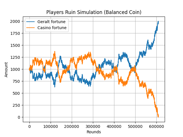
Simulation of the gambler's ruin where Geralt wins after approximately 600,000 rounds.
He explains that despite the law of large numbers, where results tend to converge towards the theoretical probability, the player is always confronted with the risk of losing everything he possesses. The gambler’s ruin, like an elusive creature, lurks in the shadows, ready to pounce on those who succumb to the call of chance without discretion. It serves as a reminder of the unpredictable nature of probability and the potential consequences of unchecked risk-taking in games of chance.

Credit: Netflix
The Secret of the Casino: Bias, Deception, and Manipulated Probabilities
In a fierce battle, the witcher emerges victorious over his adversary with unmatched grace. The masked face of the stranger is unveiled, revealing a gaze filled with admiration and surprise. With a trembling voice, he reveals his true identity as the powerful owner of the casino. The witcher is taken aback, realizing that the fortune of this man far surpasses any predictions that could have been made.

Credit: Netflix

Credit: Netflix
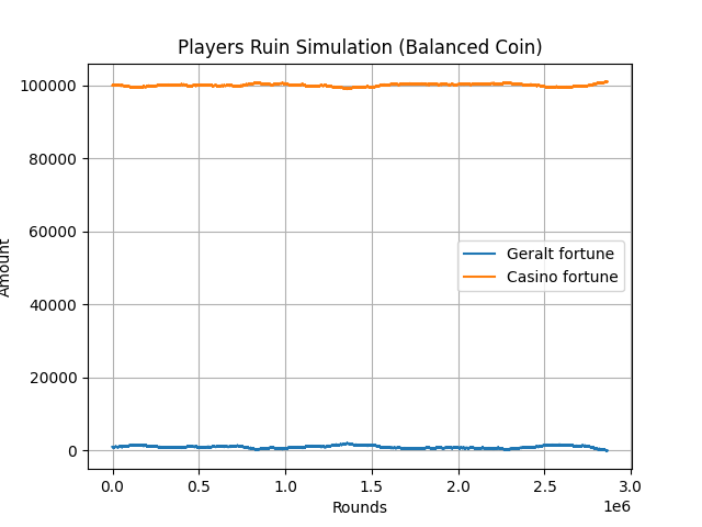
Simulation of the player's ruin when the casino has 100 times more money than Geralt.
Credit: Netflix
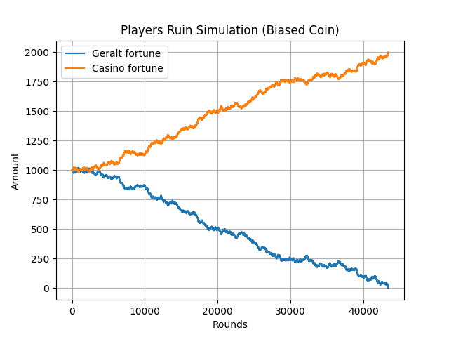
Simulation of the player's ruin with a biased coin (\(p=0.49\)).
An aura of intrigue hangs in the air as Geralt absorbs this unexpected information. He realizes that he has just unmasked a far more cunning adversary than he could have imagined. But armed with his wisdom and experience, the Witcher is already preparing to face the new challenges that lie ahead. A new quest begins, where the fate of rigged coins and unsuspecting players will intertwine with that of the Witcher, in a complex dance where the stakes are higher than ever before.
The Manipulation of Coin Tosses
The power of the concentration potion fades, and Geralt snaps out of his trance. It is at this moment that the words of the renowned magician Persi Diaconis resonate in the Witcher’s mind.
Credit: Netflix
The precision potion he possesses is a unique creation of its kind. Just a sip of this potion elevates his abilities to an extraordinary level, granting him total mastery over the coin toss. Like a machine, Geralt controls every aspect of the toss: the initial conditions, the number of rotations performed in the air, and even which side will be revealed when the coin lands. His precision in manipulating these parameters is astounding, challenging the idea that the game of coin tossing is a simple random process.
This spectacular demonstration of mastery perfectly illustrates the findings of the study conducted by Joe Keller in our reality. Indeed, this study reveals that coin tossing, although it may seem random, is actually governed by mechanical laws. When a coin is tossed with high initial velocity and strong rotation, it has a probability of landing on the same side as where it started, in nearly half of the cases. However, if we take into account precession, which is the change in the coin’s axis of rotation during its flight, the outcome can differ. If the angle between the angular momentum and the normal to the coin is less than 45 degrees, the coin will never flip and will always land on the same side.
Thanks to his precision potion, Geralt sheds light on the possibility of manipulating coin tosses in a controlled manner, creating the illusion of a random game while being aware that the results are actually determined by mechanical factors. At the heart of this manipulation lies a crucial element: the hand that tosses the coin doesn’t always hold it on the same side, alternating between head and tail. It is the unconscious randomization carried out by the person tossing the coin, as they place it on their thumb before giving it a slight initial push, that evens out the probabilities of getting head or tail. Thus, the result of the toss tends towards equality.

Credit: Netflix
Indeed, for those seeking a slight advantage, diligent training in precision tossing can enable them to master this subtle art and influence the coin to land as they desire. However, in their ingenuity, games of chance introduce another random component: another player must call “Heads” or “Tails” at the precise moment the coin flutters in the air, thus escaping all predictions.
In this enchanting romance, we can appreciate the importance of this balance between precision and randomness. Geralt of Rivia, despite his extraordinary mastery of coin tossing thanks to his precision potion, realizes that the true essence of the game lies in this unconscious randomization, which ensures fairness of probabilities. Coin tossing remains a fascinating game where uncertainty and the magic of the moment harmoniously blend, awakening in each person a curiosity tinged with mystery.
Revelations of the Coin Toss: Geralt’s Insight
In the dark twists and turns of games of chance, where the fate of eager players is decided by a simple coin toss, Geralt of Rivia, the legendary Witcher, has unveiled a troubling truth. He highlights the importance of probabilities and statistical tools to understand and analyze random situations. Despite appearances, Geralt realizes that the game of the coin toss is, in fact, a game of probabilities and chances. With his intelligence and concentration potion, he employs concepts such as the law of large numbers and the Gaussian concentration inequality to evaluate the probabilities and risks associated with coin tosses.
Although he cannot toss the coin an infinite number of times, he manages to obtain reliable estimates of the proportion of Heads and Tails using probabilistic and statistical results. Geralt’s quest also underscores the importance of prudence and self-awareness in games of chance. By being aware of probabilities and risks, Geralt makes informed decisions and minimizes the consequences of his choices.
So, whether you are a lone adventurer on the farthest reaches of the real world or a daring gambler in the depths of casinos, always remember that behind the veil of illusion lies the relentless mathematical truth. And, as Geralt has understood, sometimes the greatest victory lies in the wisdom of knowing when to step away from the gambling table, leaving behind fleeting mirages to embrace a more stable reality. One, perhaps, involving a well-deserved bath.

Credit: Netflix
Bibliography
D. Chafaï, F. Malrieu, Recueil de modèles aléatoires, 2015.
T. Bodineaux, Modélisation de phénomènes aléatoires : introduction aux chaînes de Markov et aux martingales, 2015
M. Ledoux, The concentration of measure phenomenon, 2001
I, Stewart, Do dice play god?, 2019
R. Epstein, The Theory of Gambling and Statistical Logic (Revised ed.), 1995
J. L. Coolidge, The Gambler’s Ruin. Annals of Mathematics. 10 (4): 181–192, 1909
import numpy as np
import matplotlib.pyplot as plt

def simulate_biased_coin_tosses(n, p, num_trials):
    """
    Simulates multiple trials of biased coin tosses and plots the running average.

    Args:
        n (int): Number of coin tosses in each trial.
        p (float): Probability of getting heads (biased coin).
        num_trials (int): Number of trials to simulate.
    """
    results = []

    for _ in range(num_trials):
        coin_tosses = np.random.choice([0, 1], size=n, p=[1-p, p])
        running_average = np.cumsum(coin_tosses) / np.arange(1, n + 1)
        results.append(running_average)

    # Plot the results
    for i, running_average in enumerate(results):
        plt.plot(np.arange(1, n + 1), running_average, alpha=0.5)

    # Plot the theoretical expectation (p for a biased coin)
    plt.plot(np.arange(1, n + 1), np.full(n, p), color='red', linestyle='--', label='Theoretical Expectation')

    plt.xlabel('Number of Tosses')
    plt.ylabel('Running Average')
    plt.title('Law of Large Numbers Simulation (Balanced Coin)')
    plt.legend()
    plt.grid()
    plt.show()

# Parameters
n = 100000  # Number of coin tosses in each trial
p = 0.5  # Probability of getting heads (biased coin)
num_trials = 1  # Number of trials to simulate

# Perform the simulation and visualize the results
simulate_biased_coin_tosses(n, p, num_trials)
import numpy as np
import matplotlib.pyplot as plt

def simulate_binomial_distribution(n, p, num_trials):
    """
    Simulates multiple trials of a binomial distribution and plots the histogram of outcomes.

    Args:
        n (int): Number of trials in each binomial experiment.
        p (float): Probability of success in each trial.
        num_trials (int): Number of trials to simulate.
    """
    results = np.random.binomial(n, p, size=num_trials)

    # Plot the histogram of outcomes
    plt.hist(results, bins=np.arange(n + 1) - 0.5, density=True, alpha=0.7, edgecolor='black')

    # Plot the theoretical probability mass function
    x = np.arange(n + 1)
    y = np.array([np.math.comb(n, k) * p**k * (1 - p)**(n - k) for k in x])
    plt.plot(x, y, color='red', label='Theoretical Probability')

    plt.xlabel('Number of Successes')
    plt.ylabel('Probability')
    plt.title(f'Binomial Distribution (n={n}, p={p})')
    plt.legend()
    plt.grid()
    plt.show()

# Parameters
n =10  # Number of trials in each binomial experiment
p = 0.5  # Probability of success in each trial
num_trials = 100000  # Number of trials to simulate

# Perform the simulation and visualize the results
simulate_binomial_distribution(n, p, num_trials)
# Importing libraries
import numpy as np
import pandas as pd
import seaborn as sns
from scipy.stats import norm
import matplotlib.pyplot as plt

# Function to simulate coin toss
def coin_toss(n, deviation):
    coin = np.random.choice([0, 1], size=n)  # Simulating coin toss
    proportion = np.mean(coin)  # Calculating proportion of Heads
    concentration = 2 * np.exp(-2 * n * deviation**2)  # Calculating Gaussian concentration
    return proportion, concentration

# Parameters for simulation
n_values = [10, 20, 30, 40, 50, 75, 100, 500, 1000, 10000]
deviation_values = [0.01, 0.03, 0.05, 0.07, 0.1, 0.15, 0.2, 0.25, 0.3, 0.5]

# Simulation and calculation of Gaussian concentration for each combination of parameters
results = []
for n in n_values:
    row = []
    for deviation in deviation_values:
        proportion, concentration = coin_toss(n, deviation)
        row.append(concentration)
    results.append(row)

# Creating DataFrame from results
df = pd.DataFrame(results, columns=deviation_values, index=n_values)

# Displaying results as a table
print("Number of coin tosses\t", end="")
for deviation in deviation_values:
    print(f"Deviation {deviation}\t", end="")
print()
for i, n in enumerate(n_values):
    row_str = f"{n}\t\t"
    for j, deviation in enumerate(deviation_values):
        row_str += f"{results[i][j]:.3e}\t"
    print(row_str)

# Creating heatmap with Seaborn
plt.figure(figsize=(12, 8))
sns.heatmap(data=df, annot=True, cmap="Reds", fmt=".2e", cbar=True, cbar_kws={'label': 'Gaussian concentration'})
plt.xlabel("Deviation")
plt.ylabel("Number of coin tosses")
plt.title("Gaussian concentration as a function of the deviation and the number of coin tosses")
plt.show()
# Importing libraries
import numpy as np
import pandas as pd
import seaborn as sns
from scipy.stats import norm
import matplotlib.pyplot as plt

# Function to simulate coin toss
def coin_toss(n, deviation):
    coin = np.random.choice([0, 1], size=n)  # Simulating coin toss
    proportion = np.mean(coin)  # Calculating proportion of Heads
    concentration = 2 * np.exp(-2 * n * deviation**2)  # Calculating Gaussian concentration
    return proportion, concentration

# Parameters for simulation
n_values = [10, 20, 30, 40, 100, 500, 1000]
deviation_values = [0.01, 0.03, 0.05, 0.1, 0.2]

# Simulation and calculation of Gaussian concentration for each combination of parameters
results = []
for n in n_values:
    row = []
    for deviation in deviation_values:
        proportion, concentration = coin_toss(n, deviation)
        row.append(concentration)
    results.append(row)

# Creating DataFrame from results
df = pd.DataFrame(results, columns=deviation_values, index=n_values)

# Displaying results as a table
print("Number of coin tosses\tDeviation 0.01\tDeviation 0.03\tDeviation 0.05\tDeviation 0.1\tDeviation 0.2")
for i, n in enumerate(n_values):
    row_str = f"{n}\t\t"
    for j, deviation in enumerate(deviation_values):
        row_str += f"{results[i][j]:.3e}\t"
    print(row_str)

# Creating the graph with Seaborn
sns.set(style="whitegrid")
plt.figure(figsize=(10, 6))
sns.lineplot(data=df, markers=True, dashes=False)
plt.xlabel("Number of coin tosses")
plt.ylabel("Gaussian concentration")
plt.title("Gaussian concentration as a function of the number of coin tosses and the deviation")
plt.legend(title="Deviation")
plt.show()
import numpy as np
import matplotlib.pyplot as plt

def simulate_ruin(player_a_amount, player_b_amount, win_probability):
    """
    Simulates the ruin of two players in a gambling game and returns the number of rounds played.

    Args:
        player_a_amount (int): Initial amount of money for player A.
        player_b_amount (int): Initial amount of money for player B.
        win_probability (float): Probability of winning a bet.

    Returns:
        int: Number of rounds played until one of the players goes broke.
    """
    rounds = 0

    while player_a_amount > 0 and player_b_amount > 0:
        # Simulate a round of the game
        if np.random.rand() < win_probability:
            player_a_amount += 1  # Player A wins
            player_b_amount -= 1  # Player B loses
        else:
            player_a_amount -= 1  # Player A loses
            player_b_amount += 1  # Player B wins

        rounds += 1

    return rounds

def simulate_ruin_visual(player_a_amount, player_b_amount, win_probability):
    """
    Simulates the ruin of two players in a gambling game with a biased coin and visualizes the results.

    Args:
        player_a_amount (int): Initial amount of money for player A.
        player_b_amount (int): Initial amount of money for player B.
        win_probability (float): Probability of winning a bet.
    """
    player_a_history = [player_a_amount]
    player_b_history = [player_b_amount]
    rounds = 0

    while player_a_amount > 0 and player_b_amount > 0:
        # Simulate a round of the game with a biased coin
        if np.random.rand() < win_probability:
            player_a_amount += 1  # Player A wins
            player_b_amount -= 1  # Player B loses
        else:
            player_a_amount -= 1  # Player A loses
            player_b_amount += 1  # Player B wins

        rounds += 1
        player_a_history.append(player_a_amount)
        player_b_history.append(player_b_amount)

    # Plot the results
    plt.plot(player_a_history, label='Geralt fortune')
    plt.plot(player_b_history, label='Casino fortune')
    plt.xlabel('Rounds')
    plt.ylabel('Amount')
    plt.title('Players Ruin Simulation (Balanced Coin)')
    plt.legend()
    plt.grid()
    plt.show()

# Parameters
player_a_amount = 1000  # Initial amount of money for player A
player_b_amount = 1000  # Initial amount of money for player B
win_probability = 0.5  # Probability of winning a bet (balanced coin)

# Perform the simulation and get the number of rounds played
rounds_played = simulate_ruin(player_a_amount, player_b_amount, win_probability)
print("Number of rounds played:", rounds_played)

# Perform the simulation and visualize the results
simulate_ruin_visual(player_a_amount, player_b_amount, win_probability)