How to Build a Host?
Episode I
By Jordan Moles on January 2, 2024

In the year 2051, a fortunate group of young scientists is granted the exclusive opportunity to explore the mysteries of WestWorld. Their behind-the-scenes journey takes an extraordinary turn as they are invited to a unique conference orchestrated by the enigmatic park director, Dr. Ford. At the core of this encounter lies a captivating dive into the realm of Deep Learning, offering participants an unprecedented experience and unveiling the secrets of the symbiosis between cutting-edge technology and the bold imagination of WestWorld.
At the Crossroads of Intelligence


Our ambition extends far beyond a mere recreation of the Wild West. WestWorld pushes the boundaries of imagination by introducing hosts, androids of unparalleled sophistication capable of interacting indistinguishably with our visitors. It’s not just entertainment; it’s an exploration of the deepest realms of artificial intelligence: Deep Learning.
At the heart of this technologically forged paradise, our quest aims to continually push the boundaries of what’s possible. Our hosts don’t merely replicate preprogrammed actions; they react, learn, and evolve in real-time. Nurtured for years by a vast database, we’ve trained, validated, and subjected them to tests (supervised learning), ensuring they provide a unique experience and have the ability to learn autonomously thereafter.
The neural networks that power them, drawing inspiration from the complexity of the human brain, equip them with the versatility needed to perform a variety of tasks, from driving a carriage to horseback riding, from reading to writing, from recognizing their counterparts to expressing empathy through emotion recognition. This sublime union between machine and human thought goes beyond classical Machine Learning models such as K-Nearest Neighbors, decision trees, or support vector machines. Each interaction with a visitor represents an opportunity to refine their cognitive skills (unsupervised learning), providing a unique experience at every moment, even if this aspect will not be explored in this conference.
At WestWorld, our mission extends beyond providing simple entertainment; we give birth to virtual worlds that transcend reality. For enlightened minds like yours, eminent actors in this endeavor, it’s an expedition to the frontier of technology and humanity, a fusion of artistic creativity and advanced computing power. Our goal today is to initiate you into the fundamental concepts of neural networks by introducing the multilayer perceptron and unveiling the process through which our hosts learn to recognize numbers. In an upcoming conference, we will explore in detail how they manage to identify other individuals. Get ready to embark on an adventure where the line between man and machine blurs, opening horizons as vast as imagination itself.
At the Beginning: The Biological Neuron
Numbering around 86 billion and connected by thousands or even tens of thousands of synapses, these highly specialized cells, encoded in our genetic heritage for billions of years, are called neurons.
Assembled into a network, these neurons, which we classify as “biological” in contrast to “artificial,” generate human thought and what we label as intelligence. However, they are not the only brain cells in action. Other cell types play a fundamental role and contribute to the neuronal process, with their essential presence being indispensable to the very existence of neurons.
The structure
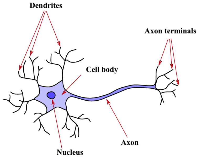
The fundamental structure of the nervous system, consisting of interconnected excitable cells, plays a crucial role in the transmission of information within our neural network. It comprises several key components that orchestrate its function.
The dendrites act as interfaces with the environment, forming the neuron’s input. In large numbers, these extensions respond to various stimuli, such as light at the eyes or pressure on the skin, generating electrical discharges, also called action potentials, directed toward the cell body. The synapse, the connection point between neurons, plays a crucial role at this juncture, where the neuron receives signals from previous neurons or from the outside. These signals, whether inhibitory or excitatory (+1 or -1), converge onto the neuron, and when their sum exceeds a critical threshold, the neuron activates, thus producing an electrical signal.
The cell body, central to the process, performs a summation of the intensity of electrical influx from all dendrites. If this sum exceeds a critical threshold, the neuron activates and generates an electrical discharge transmitted to the axon, the neuron’s single output pathway. This critical threshold, determining supra-threshold excitation, holds big significance.
The axon, as the common final pathway, branches into multiple extensions, connecting the neuron to other neurons through the following dendrites and synapses. These points of connection, anatomically represented as synaptic clefts, are essential for the transfer of information between neurons. The axon’s termination, marked by neurotransmitter vesicles, releases these chemical messengers into the synaptic cleft. In turn, the dendrite of the next neuron, equipped with receptors, binds the neurotransmitters, thus triggering the formation of an electrical current in the dendrite.
Regarding the information transmitted by the neuron, it is important to understand its electrochemical dualism. Initially created in electrical form at the dendrites in response to a stimulus, the information propagates through the cell body to the axon. At its termination, the electrical influx triggers the release of neurotransmitters, transforming the information into a chemical form at the synapse.

It is important to emphasize that this information flows in only one specific direction, from the dendrites to the axon. The dendrite captures the signal, and the axon broadcasts it, creating unidirectionality in the flow of neuronal information. This subtle electrochemical dance within the neuron forms the foundation of our understanding, thoughts, and interaction with the world around us.
How does it Works ?
As the pivot of the nervous system, it reveals itself as the master cell capable of transmitting electrochemical signals throughout the organism. These signals, resulting from depolarizations of the plasma membrane and the release of chemical molecules at connection points with other cells, form the foundation of neurotransmission.
Each neuron, dedicated to specific tasks, contributes to a complex network that enables diverse functions such as memory, motor skills, learning ease, and even speech recognition, among others.
The variety of neurons, reflecting the diversity of roles they fulfill, makes them essential actors in the complex orchestration of the functions of the nervous system. Through their extensions, the dendrites and the axon, these cells establish vital connections with innervated organs and other neurons, consolidating their central role in the functions of the nervous system.
The First Artificial Neuron in History
Ladies and gentlemen, it is now appropriate to introduce to you the famous artificial neuron, a major concept in computer science inaugurated by W. McCulloch and W. Pitt as early as 1943, a bygone era.
Although devoid of physical reality, this remarkable element provides a simple algorithmic replica of its biological counterpart, thus marking the beginning of a fascinating journey into the world of artificial intelligence.
Its Structure and Functioning
The structure of the artificial neuron is characterized by several key elements, including input and synaptic weights, the cell body, and the output. Each of these aspects contributes crucially to information processing within artificial neural networks. Let’s explore each of them in detail.
We Collect the Information
Let’s start with the input. In computer science, the input represents the data to be processed, such as a sequence of characters, an image, a gold density, or even a video.
Each artificial neuron receives a variable number of inputs from upstream neurons, which we’ll denote as X. These inputs are signals that activate the neuron and are accompanied by weights (represented by “w” for “weight”) that quantify the strength of the connection.
The set of these inputs forms the first stage of information processing by the artificial neuron.

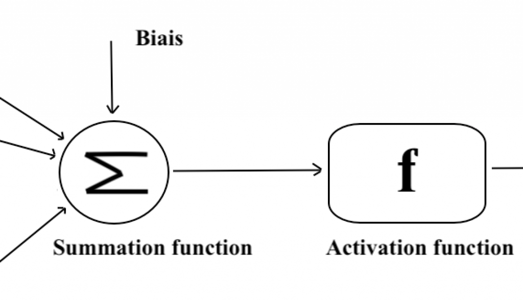
The Artificial Cell Body: a Mathematical Function
The Aggregation Phase: Inspired by the functioning of dendrites, synaptic weights are assigned to each input value, representing the relative importance of different connections to the neuron. The inputs, thus weighted, are then summed, incorporating a bias (a constant value). For now, we consider synaptic weights of either +1 (excitatory) or -1 (inhibitory), but we will generalize this later.
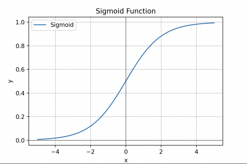
The Activation Phase: Following the aggregation phase, an activation function determines whether the neuron should be activated. Initially, we choose a threshold function (known as the Heaviside step function). This function returns an output \(y=1\) if the previous weighted sum exceeds a threshold value and 0 otherwise (here is a graphical representation).
Activation functions play a essential role in information processing and can take various forms, including the step function, the sigmoid function (remember the sigmoid), the rectified linear unit (ReLU) function, or even the hyperbolic tangent function.


Processed Information
The output of the artificial neuron is the final result of the information processing contained in the input data X, either y=0 (activated) or y=1 (deactivated). It can be transmitted to other neurons, thus forming a complex chain of calculations that characterizes the overall operation of artificial neural networks.


This initial model of the artificial neuron was later termed the “Threshold Logic Unit” due to its ability to process only logical inputs of either 0 or 1. Researchers successfully demonstrated that this model could replicate certain logical functions such as the AND and OR gates. By interconnecting multiple units in a manner similar to the connections between neurons in our brains, it seemed possible to solve virtually any boolean logic problem.
Despite the excessive enthusiasm generated by this announcement, I want to assure you that, at the time, a significant portion of the scientific community believed that we could develop artificial intelligences capable of entirely replacing humans.
Scientist in the audience, looking at the hosts next to Dr. Ford: “They weren’t entirely wrong!” Laughter in the room.
Dr. Ford resumes with a smile: Indeed, not entirely wrong, just that their timeline wasn’t suited to this prediction. Nevertheless, this anticipation did not materialize directly. Although this model laid the groundwork for what is now known as Deep Learning, it had several limitations, notably the absence of a learning algorithm. Thus, users had to manually determine the values of the parameters “W” if they wished to apply this model to real-world applications.
A Simple Example
Normally, these are basics, but let’s start with a brief explanation of Boolean algebra for the two scientists in the background.
Boolean algebra, named after the British mathematician George Boole, is a branch of mathematics that focuses on the representation and manipulation of logical information through operations on variables called booleans. These variables can only take two values, typically denoted as 0 and 1, representing the states false (no) and true (yes), respectively.
Widely used in computer science, electronics, and other information processing-related fields, Boolean algebra is fundamental to the design of logical circuits, algorithms, and serves as the basis for propositional logic.
In Boolean algebra, the fundamental operations are logical AND, logical OR, and logical NOT. These operations apply to pairs of Boolean variables and produce a Boolean result.
An Example within an Example
Now, to better understand these operations, let’s consider an example of a room with a switch A and a sensor B detecting the presence of people, controlling the lighting.
Switch A AND Sensor B (A AND B):
– If switch A is on (A = 1) AND sensor B detects people (B = 1), then condition C “the light turns on” is TRUE (C = 1).
– If switch A is off (A = 0), even if sensor B detects people (B = 1), condition C is FALSE (C = 0).
– If switch A is on (A = 1) but sensor B does not detect people (B = 0), condition C is also FALSE (C=0).
– If both switch A and sensor B are off (A=0 and B=0), condition C is FALSE (C=0).
Switch A OR Sensor B (A OR B):
– If switch A is on (A = 1) OR sensor B detects people (B = 1), then condition C is TRUE (C=1).
– If switch A is off (A = 0) OR sensor B detects people (B = 1), then condition C is TRUE (C=1).
– If both, if switch A is on (A = 1) or sensor B does not detect people (B = 0), then the condition is TRUE (C=1).
– If switch A is off (A = 0) or sensor B does not detect people (B=0), then condition C is FALSE (C = 0).
In these examples, the AND operation requires the switch to be on and people to be detected for the condition to be true. Conversely, the OR operation requires either the switch to be on or people to be detected for the condition to be true.
We can summarize everything in these two tables:
| A | B | A AND B |
|---|---|---|
| 0 | 0 | 0 |
| 0 | 1 | 0 |
| 1 | 0 | 0 |
| 1 | 1 | 1 |
| A | B | A OR B |
|---|---|---|
| 0 | 0 | 0 |
| 0 | 1 | 1 |
| 1 | 0 | 1 |
| 1 | 1 | 1 |
These basic operations can be combined to form more complex logical expressions, allowing for the representation of conditions (not just two, as in the previous example) and logical reasoning.
Boolean algebra finds practical applications in the design of logic circuits, control systems, computer science, and other fields where binary logic is used to model states and decisions.
Revenons au Neurone
The scientist from the background raises his hand to ask a question: “But what does a neuron have to do with Boolean algebra?”
Dr. Ford delves into the explanations: “Let’s simplify and consider a formal neuron that simply accepts two input variables \(x_1\) and \(x_2\) arranged in an input vector (this is the information the neuron receives).
\begin{equation*} \mathbf{X}=\left[ \begin{array}{c} x_{1} \\ x_{2} \end{array} \right]. \end{equation*}
Knowing that the inputs can only take the values 0 or 1 in our case, we have only 4 possible input vectors:
\begin{equation*} \left[ \begin{array}{c} 0 \\ 0 \end{array} \right]\quad \left[ \begin{array}{c} 0 \\ 1 \end{array} \right]\quad \left[ \begin{array}{c} 1 \\ 0 \end{array} \right]\quad \left[ \begin{array}{c} 1 \\ 1 \end{array} \right] \end{equation*}”
They are also defined by two synaptic parameters \(w_1\) and \(w_2\), which are also placed in a vector, denoted as \(\mathbf{W}\).
\begin{equation*} \mathbf{W}=\left[ \begin{array}{c} w_{1} \\ w_{2} \end{array} \right]. \end{equation*}
These can take values of either 1 or -1. So, as before, we have only 4 possible weight vectors:
\begin{equation*} \left[ \begin{array}{c} -1 \\ -1 \end{array} \right]\quad \left[ \begin{array}{c} -1 \\ 1 \end{array} \right]\quad \left[ \begin{array}{c} 1 \\ -1 \end{array} \right]\quad \left[ \begin{array}{c} 1 \\ 1 \end{array} \right] \end{equation*}

Now we can begin the aggregation phase, which first takes an input, associates it with a corresponding weight, sums it up, and adds a bias denoted as b. Here is the result:
\[ \Sigma = w_1 x_1 + w_2 x_2 + b \]
We place all of this in a table.
Then we move on to the activation phase, meaning we introduce the obtained value \(\Sigma\) into our threshold function, denoted as H, which determines the neuron’s output as follows:
\[ y = H(\Sigma + b) \]
Applying a similar reasoning, we observe that a neuron with a single input can either have no effect (identity neuron) or perform a logical NOT operation.
By establishing a connection with Boolean algebra, we have demonstrated how this model can perform fundamental logical operations, such as OR and AND.
However, despite its advancements, this model alone has two major limitations: firstly, it is limited to simple operations, and secondly, it lacks any learning mechanism. As illustrated earlier, the only operations we can perform are OR and AND, and we must manually determine the weight values to carry out these specific logical operations. These limitations have motivated the further development of more sophisticated models in the field of Deep Learning. By networking these neuron models, we gain the ability to solve virtually any Boolean logic problem. Furthermore, if we allow the model to learn autonomously, it becomes possible to address more complex issues and significantly expand its capabilities.
The advent of the Perceptron
The perceptron, designed by the American psychologist Frank Rosenblatt around fifteen years after the introduction of the formal neuron concept by McCulloch and Pitt, represents a significant advancement with the introduction of the first Deep Learning learning algorithm.
The perceptron model shares a striking similarity with the one we have just studied. In fact, the only difference between the perceptron and the previous formal neuron lies in the addition of a learning algorithm that enables it to determine the values of its parameters W, in order to achieve the desired outputs y, thus eliminating the need for manual search by humans.
F. Rosenblatt drew inspiration from Hebb’s law in neuroscience, suggesting that the strengthening of synaptic connections between two biological neurons occurs when they are excited together, a phenomenon known as the “cells that fire together, wire together” principle. This synaptic plasticity is crucial in the construction of memory and learning.
The Hebb's Law
The learning algorithm of the perceptron involves training the artificial neuron on reference data (X, y). With each activation of the input X simultaneously with the presence of the output y in the data, the parameters W are strengthened. F. Rosenblatt formulated this idea with the following equation:
\[ W^* = W + \delta(y_{\text{ref}} – y)X \]
where the new weights \( W^* \) are updated with a learning rate \( \delta \). \( y_{\text{ref}} \) is the reference output, y is the output produced by the neuron, and X is the neuron’s input.
This formula adjusts the weights to minimize the difference between the expected output and the output produced by the neuron. Thus, if the neuron produces an output different from the expected one (e.g., y=0 instead of y=1), the weights associated with the activated inputs are increased. This process continues until the neuron’s output converges to the expected output.
Model Limitations
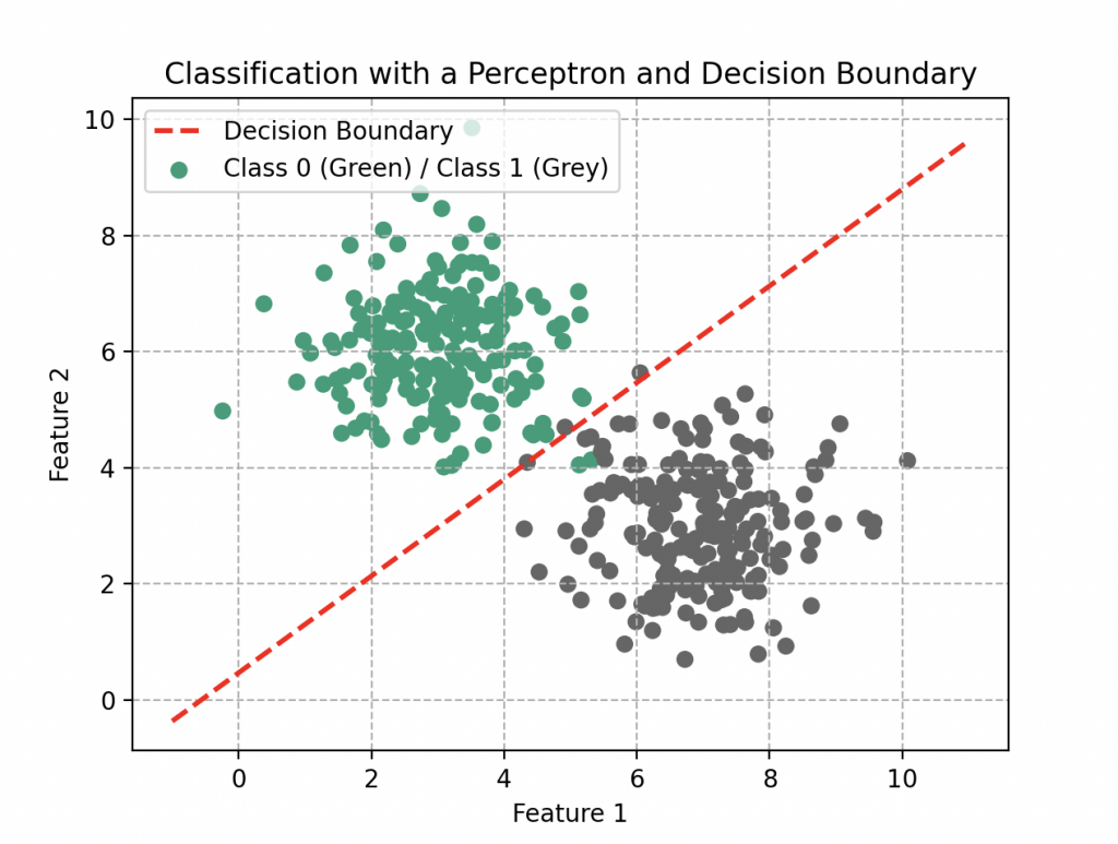
Ladies and gentlemen of the scientific community, let us now consider a perceptron composed solely of two inputs \(x_1\) and \(x_2\). Its aggregation function is thus \(f(x_1, x_2) = w_1x_1 + w_2x_2\), and, due to its form, it can model linear relationships. However, this simplicity comes with limitations when faced with nonlinear problems.
Dr. Ford astutely points out, “The perceptron, at its core, is like a tool with a narrow perspective. It may succeed in making rough predictions, but it struggles to grasp the complexity of nonlinear relationships present in the real world.”
A scientist from the audience, displaying a profound understanding, remarks, “It’s like trying to predict the behavior of a circle by drawing only a line with a ruler.”
Dr. Ford, smiling, responds, “Exactly! That’s why we are exploring more complex approaches to model the richness of relationships.”
A few more Perceptrons
To overcome this initial problem, let’s first introduce three perceptrons that we will connect together. The first two will each receive inputs \(x_1\) and \(x_2\), perform their calculations based on their parameters, and then send an output \(y\) to the third perceptron. The third one will also perform its own calculations to produce a final output.
Try programming three neurons as described above, and you can plot the graphical representation of the final output based on the inputs \(x_1\) and \(x_2\). This will yield a nonlinear model, much more interesting.
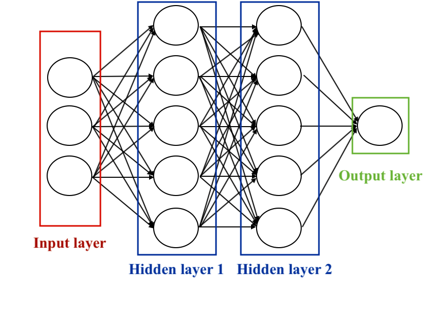
This model will then be your first artificial neural network, consisting of 3 neurons distributed across two layers: an input layer and an output layer. You can add as many layers and neurons as you want, but the more you add, the more computational time and resources will be required for simulating complex results. You can also change the topology, meaning the nature of connections between neurons. This will depend on the problem at hand. That’s what we will explore next.
Neural Networks
Neural networks, also known as artificial neural networks, are computational models inspired by the structure and functioning of the human brain. They consist of interconnected artificial neurons organized into layers. Each neuron receives inputs, performs processing operations, and then produces an output. These outputs are then transmitted to the neurons in the next layer, creating a layered architecture.
Neural networks typically include three main types of layers:
1. Input Layer: Receiving input data from the system, each node in this layer represents a feature or input variable.
2. Hidden Layers: These layers perform data transformation operations. Each node in a hidden layer takes inputs, applies weights and biases, and produces an output. They are really important for the network to learn complex representations of the data.
3. Output Layer: Producing the final prediction or classification, this layer synthesizes the information learned by the hidden layers to generate the ultimate output.
The choice of hidden units is an active area of research in machine learning. The number of hidden layers is referred to as the depth of the neural network. The question of how many layers make a network “deep” does not have a single answer. Generally, deeper networks have the capacity to learn more complex functions.
There are several types of neural networks based on the topology of connections between neurons. The topology can vary depending on the specific architecture of the network, but some regularities are commonly observed. Here are some examples of topologies:
• Multi-layer perceptron (MLP): Each neuron in a layer is connected to all neurons in the next layer. It is a simple configuration used, notably, for image classification.
• Convolutional Neural Network (CNN): Specialized in image processing, it uses filters to analyze local parts, reducing the number of parameters and extracting important features.
• Recurrent Neural Network (RNN): Designed to process sequential data, it uses recurrent connections to consider the temporal sequence of data.
• Long Short-Term Memory (LSTM): An extension of RNNs, LSTMs handle longer sequences by mitigating the vanishing gradient problem.
• The Autoencoder Network: Intended for unsupervised learning, the autoencoder network consists of an encoder layer and a decoder layer. Its goal is to reproduce the input while generating a latent representation. Emphasis is on dimension reduction, particularly useful with large volumes of data. By substituting this data with a representation in a lower-dimensional space, processor efficiency is optimized, enhancing the model’s effectiveness (discussed in another article).
• Residual Neural Network (ResNet): Introduced to address the vanishing gradient problem, ResNets use residual connections to facilitate learning of deeper representations.
In this exploration, we will particularly focus on feedforward neural networks. It is the first type of artificial neural network, the simplest one, where information moves only forward, from input nodes to output nodes, without cycles or loops (it is said to be acyclic, distinguishing it from recurrent networks). The single perceptron we have already seen, and its well-known extension, the multi-layer perceptron, which we will delve into shortly.
But by the way, I forgot, how do we train a neural network to do what we ask of it, meaning how do we find the parameters \(w\) and \(b\) to obtain the right model?
The entire audience remains silent.
Don’t worry; we are about to discuss that now.
Cognitive Programming of Hosts for Handwritten Digit Recognition: The Multilayer Perceptron
Before our hosts can excel in more advanced tasks, such as recognizing humans or even emotions, it is imperative to initiate them into the fundamentals, starting with the recognition of handwritten digits because, as the proverb goes, “Before learning to run, one must learn to walk.”
To guide them in this (supervised) learning, we use a series of images of digits, each visually representing the correspondence between the handwritten form and the respective digit.
Next, our hosts are challenged to recognize the presented digits.
This classification model forms the first artificial neural network for our hosts, comprising an input layer, several hidden layers (to be determined), and an output layer. Such a multilayer network, where complexity can be increased by adding more layers and neurons, but it will require more computational time.
Now, let’s explore the process to which our hosts are subjected during their programming to master this task.
Assimilation des Données d'Entraînement (DataSet)
Our hosts are supplied with training data, consisting of 60,000 examples of 28 pixel by 28 pixel resolution grayscale images of handwritten digits and their respective correspondences. This data is needed for teaching hosts to generalize from existing examples. And 10,000 test images of the same format to examine them, i.e. how well they have classified the images. Here are the numbers from 0 to 9:


Such images are simply arrays of data containing numbers from 0 to 255. Each of the 60,000 arrays is “flattened” to form 60,000 X vectors with 784 coordinates corresponding to the total number of pixels in an image with a y label between 0 and 9.
Building the Cognitive Model
The cognitive model represents the structure of the neural network in our hosts’ minds, encompassing aspects such as the number of layers, the number of neurons per layer, learning parameters (W and b), and even activation functions. Model design is highly dependent on the specific nature of the task at hand.
Weights and biases will undergo continuous adjustments throughout training to minimize the error between model predictions and expected outputs. Appropriate initialization and updating of these parameters is useful to optimize network performance. Other parameters such as the number of layers and the number of neurons will be adjusted manually to find the most efficient model within a reasonable timeframe and without consuming excessive resources, as it is undesirable for a host to take 30 seconds to recognize a handwritten digit, or to be inactive during this task.
Forward propagation
The first step in this cognitive process is forward propagation: the host brain circulates information from the pixels of the first layer to the last, producing an output y (the handwritten digit label).
Let’s analyze how it works.
• The input layer consists of just 784 neurons, each analyzing one pixel of the image. It has no parameters.
• The hidden layers (sigmoid): next, we endow our hosts with two hidden layers, each comprising 100 neurons with a sigmoid activation function.
The output of the first layer is a vector \(A^1\) containing 100 coordinates (one for each neuron). The calculations carried out for each element are simple and are based on the perceptron model: we calculate the aggregation function and then apply the activation function to it.

We write everything compactly in matrix form.
\begin{align*}
Z^{1} &= W^{1}\cdot X+b^1\\
A^{1} &= \frac{1}{1+\exp{(-Z^{1})}}
\end{align*}
The second hidden layer provides a vector \(A^2\) also containing 100 coordinates. We do the same for the second layer
\begin{align*}
Z^{2} &= W^{2}\cdot A^{1}+b^2\\
A^{2} &= \frac{1}{1+\exp{(-Z^{2})}}
\end{align*}
• The output layer: Finally, since the aim is to classify numbers from 0 to 9, an output layer of 10 neurons, accompanied by a softmax activation function, is more than sufficient.
\begin{align*}
Z^{3} &= W^{3}\cdot A^{2}+b^2\\
A^{2} &= \frac{1}{1+\exp{(-Z^{3})}}
\end{align*}
The softmax function assigns probabilities to each possible class. For each input image, it assigns a probability of belonging to class 0, 1, 2, …, up to 9. Here’s an example
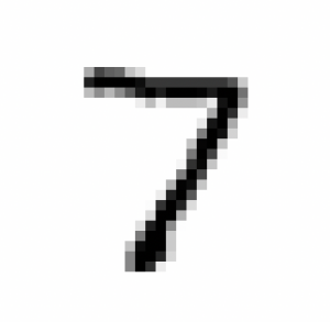

| Digits | 0 | 1 | 2 | 3 | 4 | 5 | 6 | 7 | 8 | 9 |
|---|---|---|---|---|---|---|---|---|---|---|
| Probabilities | 0.00000028 | 0.00000000023 | 0.000017 | 0.000070 | 0.00000000019 | 0.00000030 | 0.000000000018 | 0.99 | 0.0000018 | 0.000022 |
According to this table, there’s virtually no doubt that this number is 99% 7, so the host will assign it this number. In general, the host will assign the image the label with the highest probability.
This function therefore allows results to be interpreted as the confidence of the model in each class, and facilitates decision-making in the context of a multiclass classification task.
Cognitive Error Analysis: The Cost Function
In the second phase, the host neural network analyzes the error between the model’s output y (its prediction) and the expected reference output (y_{text{ref}}). This evaluation is carried out using a cost function frequently used in classification tasks, including handwritten digit recognition. In this case, it’s the categorical cross-entropy, which we’ve already encountered (in another form).

We recall its expression:
\begin{align*}L(W,b)=-\frac{1}{n}\sum_{k=1}^n\left[y^{(k)}\log{y_{\text{ref}}}+\left(1-y^{(k)}\right)\log{\left(1-y_{\text{ref}}\right)}\right].\end{align*}
In general, \(y_{ref}\) can be the final output but also any neuron layer output \(A^{i}\) with i the i-th layer which we place in an array named \(\mathbf{A}\). This gives the following matrix formula:
\begin{align*}L(W,b)=-\frac{1}{n}\left[\mathbf{y}\log{\mathbf{A}}+\left(1-\mathbf{y}\right)\log{\left(1-\mathbf{A}\right)}\right].\end{align*}
This is a fundamental element in the cognitive analysis of the model, and measures the difference between the probabilities predicted by the model and the actual probabilities of the classes. Its aim is to appropriately quantify the discrepancy between the neural network’s predictions and the true labels associated with the digit images. Efficient minimization of this cost function during training helps to fine-tune the model parameters for better performance. de chiffres. Une minimisation efficace de cette fonction coût lors de l’entraînement contribue à affiner les paramètres du modèle pour une meilleure performance.
Mechanisms of Comprehension
The third step is backpropagation. The hosts measure how this cost function varies in relation to each layer of the model, working backwards from the last to the first. In other words, they will analyze the error of the output and the penultimate layer, then the penultimate layer and the penultimate layer and so on, all the way back to the input layer.
In short, we need to calculate how the error propagates from the output to the input in order to reduce it. On this network with two hidden layers, this results in 6 terrifying expressions (if you remember just the previous sentence, that’s fine):
Starting with the last one (from the exit to the second one)
\begin{align*}
\frac{\partial L(\mathbf{W},b)}{\partial \mathbf{W}^3} =\frac{\partial L}{\partial \mathbf{A}^3} \times \frac{\partial \mathbf{A}^3}{\partial \mathbf{Z}^3} \times \frac{\partial \mathbf{Z}^3}{\partial \mathbf{W}^3}
\end{align*}
\begin{align*}
\frac{\partial L(\mathbf{W},b)}{\partial \mathbf{b}^3} =\frac{\partial L}{\partial \mathbf{A}^3} \times \frac{\partial \mathbf{A}^3}{\partial \mathbf{Z}^3} \times \frac{\partial \mathbf{Z}^3}{\partial \mathbf{b}^3}
\end{align*}
penultimate (second to first)
\begin{align*}\frac{\partial L(\mathbf{W},b)}{\partial \mathbf{W}^2} =\frac{\partial L}{\partial \mathbf{A}^3} \times \frac{\partial \mathbf{A}^3}{\partial \mathbf{Z}^3} \times \frac{\partial \mathbf{Z}^3}{\partial \mathbf{A}^2}\times\frac{\partial \mathbf{A}^2}{\partial \mathbf{Z}^2} \times \frac{\partial \mathbf{Z}^2}{\partial \mathbf{W}^2}\end{align*}
\begin{align*}\frac{\partial L(\mathbf{W},b)}{\partial \mathbf{W}^2} =\frac{\partial L}{\partial \mathbf{A}^3} \times \frac{\partial \mathbf{A}^3}{\partial \mathbf{Z}^3} \times \frac{\partial \mathbf{Z}^3}{\partial \mathbf{A}^2}\times\frac{\partial \mathbf{A}^2}{\partial \mathbf{Z}^2} \times \frac{\partial \mathbf{Z}^2}{\partial \mathbf{}^2}\end{align*}
and finally the Input (from the first to the input)
\begin{align*}\frac{\partial L(\mathbf{W},b)}{\partial \mathbf{W}^1} =\frac{\partial L}{\partial \mathbf{A}^3} \times \frac{\partial \mathbf{A}^3}{\partial \mathbf{Z}^3} \times \frac{\partial \mathbf{Z}^3}{\partial \mathbf{A}^2}\times\frac{\partial \mathbf{A}^2}{\partial \mathbf{Z}^2}\times \frac{\partial \mathbf{Z}^2}{\partial \mathbf{A}^1}\times\frac{\partial \mathbf{A}^1}{\partial \mathbf{Z}^1} \times \frac{\partial \mathbf{Z}^1}{\partial \mathbf{W}^1} \end{align*}
\begin{align*}\frac{\partial L(\mathbf{W},b)}{\partial \mathbf{b}^1} =\frac{\partial L}{\partial \mathbf{A}^3} \times \frac{\partial \mathbf{A}^3}{\partial \mathbf{Z}^3} \times \frac{\partial \mathbf{Z}^3}{\partial \mathbf{A}^2}\times\frac{\partial \mathbf{A}^2}{\partial \mathbf{Z}^2}\times \frac{\partial \mathbf{Z}^2}{\partial \mathbf{A}^1}\times\frac{\partial \mathbf{A}^1}{\partial \mathbf{Z}^1} \times \frac{\partial \mathbf{Z}^1}{\partial \mathbf{b}^1} \end{align*}

Optimisation Mentale
Finally, the fourth stage is mental optimization. Hosts mentally adjust each model parameter using gradient descent (remember that? see the article Wall-E: The Little Gold Miner), before returning to the first stage, forward propagation, to start a new training cycle.
\begin{align*}\mathbf{W^*}=\mathbf{W}-\delta \frac{\partial }{\partial \mathbf{b}}L(\mathbf{W},\mathbf{b})\\
\mathbf{W^*}=\mathbf{W}-\delta \frac{\partial }{\partial \mathbf{W}}L(\mathbf{W},\mathbf{b})
\end{align*}
where \(\delta\) is the learning rate of all neurons.
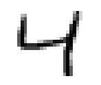
In summary, this process enables our hosts to master handwritten digit recognition to some extent, with a success rate of around 83%, although this performance is not exceptional. Here are some of the mistakes our guests make:
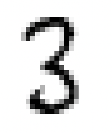


Clearly, some handwritten numbers can be confusing, even to the human eye, while others seem to be unmistakably identifiable, like the 3 above.

So, by adjusting a few parameters, it becomes relatively easy to significantly improve the model’s performance and reach 94% accuracy, a key skill in their journey towards acquiring more advanced cognitive tasks.
As our guests progress, they’ll broaden their scope of expertise, unlocking new possibilities for more immersive experiences at Westworld.
The Hosts of Westworld: From Numbers to Faces.
In conclusion, my dear guests, our first exploration into the mysteries of Deep Learning ends here. I’m delighted to have revealed a number of concepts to you, including formal neurons, perceptrons and multi-layer perceptrons. We’ve analyzed a concrete example where the hosts of Westworld, through their processors, have acquired the ability to recognize and interpret handwritten numbers with disconcerting accuracy.
But make no mistake, this neural network alone is far from sufficient when the world to be analyzed has a higher resolution. The number of training parameters that had to be adjusted for our multi-layer perceptron (there were many! 89,610 parameters) of just two hidden layers of 100 neurons was relatively small to be run on low-power machines. Now imagine simulating such a model with hundreds of layers and thousands of neurons per layer. It would be impossible! This is why other techniques have been developed, such as convolutional neural networks, which use filters to analyze characteristic elements of the image.
Finally, and I’ll leave it at that, don’t visualize an artificial intelligence that discerns faces, complex objects or emotions as “intelligent”. For even if hosts seem to come strikingly close to humanity in their interactions, let’s always remember that they are nothing more than machines.
Dr. Ford - "Remember, hosts are not real. They are not conscious."

Bibliography
F. Rosenblatt, The Perceptron, A perceiving and recognizing automaton, Cornell Aeronautical Laboratory, 1957
F. Rosenblatt, The Perceptron: A Probabilistic Model For Information Storage And Organization in the Brain, Psychological Review, vol. 65, no 6, 1958
M. Tommasi, Le Perceptron, Apprentissage automatique : les réseaux de neurones, cours à l’université de Lille 3.
D.B. Parker, Learning Logic , Massachusetts Institute of Technology, Cambridge MA, 1985.
G. Saint-Cirgue, Machine Learnia, Youtube Channel.
USI Events, Deep learning, Yann LeCun on Youtube.
Note: for more information on the code provided, please visit GitHub. Link in the footer!
import numpy as np
import matplotlib.pyplot as plt

# Set the random seed for reproducibility
np.random.seed(42)

# Generate points for class 0
class0_points = np.random.normal(loc=[3, 6], scale=[1, 1], size=(200, 2))

# Generate points for class 1
class1_points = np.random.normal(loc=[7, 3], scale=[1, 1], size=(200, 2))

M0 = np.zeros((class0_points.shape[0], 1))
M1 = np.ones((class1_points.shape[0], 1))

X = np.concatenate([class0_points, class1_points], axis=0)
y = np.concatenate([M0, M1], axis=0)


# Create an initialization function to initialize parameters W and b of our model
def initialization(X):
    np.random.seed(seed=0)
    W = np.random.randn(X.shape[1], 1)
    b = np.random.randn(1)
    return W, b

W, b = initialization(X)

print(W.shape)

# Next, create an iterative algorithm where we repeat the following functions in a loop:

# Start with the function that represents our artificial neuron model, where we find the function Z = X.W + b and the activation function A
def model(X, W, b):
    Z = X.dot(W) + b
    A = 1 / (1 + np.exp(-Z))
    return A

A = model(X, W, b)

# Next, create an evaluation function, i.e., the cost function that evaluates the model's performance by comparing the output A to the reference data y
def log_loss(A, y):
    return (1 / len(y)) * np.sum(-y * np.log(A) - (1 - y) * np.log(1 - A))

# In parallel, calculate the gradients of this cost function
def gradients(A, X, y):
    dW = (1 / len(y)) * np.dot(X.T, A - y)
    db = (1 / len(y)) * np.sum(A - y)
    return dW, db

dW, db = gradients(A, X, y)

print(dW.shape)
print(db.shape)

# Finally, use these gradients in an update function that updates the parameters W and b to reduce the model's errors
def update(dW, db, W, b, learning_rate):
    W = W - learning_rate * dW
    b = b - learning_rate * db
    return W, b

# Create a prediction function
def predict(X, W, b):
    A = model(X, W, b)
    return A >= 0.5

# Create an artificial neuron
def artificial_neuron(X, y, learning_rate=0.1, n_iter=100):
    # Initialize W, b
    W, b = initialization(X)

    # Visualize the loss
    Loss = []

    # Create a training loop
    for i in range(n_iter):
        A = model(X, W, b)
        Loss.append(log_loss(A, y))
        dW, db = gradients(A, X, y)
        W, b = update(dW, db, W, b, learning_rate)

    # Calculate predictions for all data
    y_pred = predict(X, W, b)

    # Display the performance of our model (e.g., accuracy), comparing the reference data y with our predictions
    # print(accuracy_score(y, y_pred))

    # Visualize the loss to see if our model has learned well
    plt.plot(Loss)
    plt.grid(ls='--')
    plt.show()
    return W, b

# Train the artificial neuron
W, b = artificial_neuron(X, y)

# Test on new data
new_data = np.array([6, 4])

plt.scatter(X[:, 0], X[:, 1], c=y, cmap='Dark2', label='Class 0 (Blue) / Class 1 (Orange)')
plt.scatter(new_data[0], new_data[1], c='red', label='New Data (Red)')
plt.title('Classification with an Artificial Neuron')
plt.xlabel('Feature 1')
plt.ylabel('Feature 2')
plt.grid(ls='--')
plt.legend()
plt.show()

prediction = predict(new_data, W, b)
print(f"Prediction for new data: {prediction}")

# Create the decision boundary
x0 = np.linspace(-1, 11, 100)
x1 = (-W[0] * x0 - b) / W[1]

plt.plot(x0, x1, c='red', lw=2, ls='--', label='Decision Boundary')
plt.scatter(X[:, 0], X[:, 1], c=y, cmap='Dark2', label='Class 0 (Green) / Class 1 (Grey)')
plt.title('Classification with a Perceptron and Decision Boundary')
plt.xlabel('Feature 1')
plt.ylabel('Feature 2')
plt.grid(ls='--')
plt.legend()
plt.show()
import numpy as np
import matplotlib.pyplot as plt
from tqdm import tqdm
from sklearn.metrics import log_loss, accuracy_score
from keras.datasets import mnist
from sklearn.preprocessing import OneHotEncoder

# Load MNIST data
(X_train, y_train), (X_test, y_test) = mnist.load_data()


# Display one image for each digit
fig, ax = plt.subplots(nrows=1, ncols=10, figsize=(20, 4))
for digit in range(10):
    digit_indices = np.where(y_train == digit)[0]
    ax[digit].imshow(255 - X_train[digit_indices[0]], cmap='gray')
    ax[digit].set_title(f'Digit {digit}')
    ax[digit].axis('off')

plt.tight_layout()
plt.show()


# Reshape and normalize input data
X_train_reshape = X_train.reshape(X_train.shape[0], -1) / 255.0
X_test_reshape = X_test.reshape(X_test.shape[0], -1) / 255.0

# Transpose labels if needed
y_train = y_train.reshape(-1, 1)
y_test = y_test.reshape(-1, 1)

# One-hot encode labels
encoder = OneHotEncoder(sparse=False, categories='auto')
y_train_onehot = encoder.fit_transform(y_train)
y_test_onehot = encoder.transform(y_test)

# Select a subset of data
m_train = 5000
m_test = 1000

X_train_reshape = X_train_reshape[:m_train, :]
X_test_reshape = X_test_reshape[:m_test, :]
y_train_onehot = y_train_onehot[:m_train, :]
y_test_onehot = y_test_onehot[:m_test, :]

print(X_train_reshape.shape)
print(X_test_reshape.shape)
print(y_train_onehot.shape)
print(y_test_onehot.shape)


# Neural network initialization function
def initialization(dimensions):
    np.random.seed(seed=0)
    parameters = {}
    C = len(dimensions)
    for c in range(1, C):
        parameters['W' + str(c)] = np.random.randn(dimensions[c], dimensions[c-1])
        parameters['b' + str(c)] = np.random.randn(dimensions[c], 1)
    return parameters

# Neural network forward propagation function
def forward_propagation(X, parameters):
    activations = {'A0': X}
    C = len(parameters) // 2
    for c in range(1, C + 1):
        Z = parameters['W' + str(c)].dot(activations['A' + str(c-1)]) + parameters['b' + str(c)]
        activations['A' + str(c)] = 1 / (1 + np.exp(-Z))
    return activations

# Neural network backpropagation function
def back_propagation(X, y, activations, parameters):
    m = y.shape[1]
    C = len(parameters) // 2
    dZ = activations['A' + str(C)] - y
    gradients = {}
    for c in reversed(range(1, C + 1)):
        gradients['dW' + str(c)] = (1/m) * np.dot(dZ, activations['A' + str(c-1)].T)
        gradients['db' + str(c)] = (1/m) * np.sum(dZ, axis=1, keepdims=True)
        if c > 1:
            dZ = np.dot(parameters['W' + str(c)].T, dZ) * activations['A' + str(c-1)] * (1 - activations['A' + str(c-1)])
    return gradients

# Neural network update function
def update(gradients, parameters, learning_rate):
    C = len(parameters) // 2
    for c in range(1, C + 1):
        parameters['W' + str(c)] = parameters['W' + str(c)] - learning_rate * gradients['dW' + str(c)]
        parameters['b' + str(c)] = parameters['b' + str(c)] - learning_rate * gradients['db' + str(c)]
    return parameters

# Neural network prediction function
def predict(X, parameters):
    activations = forward_propagation(X, parameters)
    C = len(parameters) // 2
    Af = activations['A' + str(C)]
    return (Af >= 0.5).astype(int)

# Neural network training function
def neural_network(X, y, hidden_layers=(100, 100), learning_rate=0.1, n_iter=1000):
    np.random.seed(0)
    dimensions = [X.shape[0]] + list(hidden_layers) + [y.shape[0]]
    parameters = initialization(dimensions)
    train_loss = []
    train_acc = []
    for i in tqdm(range(n_iter)):
        activations = forward_propagation(X, parameters)
        gradients = back_propagation(X, y, activations, parameters)
        parameters = update(gradients, parameters, learning_rate)
        if i % 10 == 0:
            C = len(parameters) // 2
            train_loss.append(log_loss(y, activations['A' + str(C)]))
            y_pred = predict(X, parameters)
            current_accuracy = accuracy_score(y.flatten(), y_pred.flatten())
            train_acc.append(current_accuracy)
    plt.figure(figsize=(12, 4))
    plt.subplot(1, 2, 1)
    plt.plot(train_loss, label='train loss')
    plt.legend()
    plt.subplot(1, 2, 2)
    plt.plot(train_acc, label='train acc')
    plt.legend()
    plt.show()
    return parameters

# Train the neural network
parameters = neural_network(X_train_reshape.T, y_train_onehot.T, hidden_layers=(100, 100), learning_rate=0.1, n_iter=5000)

# Predict on test data
y_pred = predict(X_test_reshape.T, parameters)

# Print accuracy on test data
test_accuracy = accuracy_score(y_test_onehot.flatten(), y_pred.flatten())
print(f"Test Accuracy: {test_accuracy}")
import numpy as np
import tensorflow as tf
import keras
import matplotlib.pyplot as plt
from keras.datasets import mnist


# Load MNIST data
(X_train, y_train), (X_test, y_test) = mnist.load_data()

# Display one image for each digit
fig, ax = plt.subplots(nrows=1, ncols=10, figsize=(20, 4))
for digit in range(10):
    digit_indices = np.where(y_train == digit)[0]
    ax[digit].imshow(255 - X_train[digit_indices[0]], cmap='gray')
    ax[digit].set_title(f'Digit {digit}')
    ax[digit].axis('off')

plt.tight_layout()
#plt.show()

# Reshape and normalize input data
X_train = X_train/ 255.0
X_test = X_test / 255.0


hidden1 = 100
hidden2 = 100

model = keras.Sequential([
    keras.layers.Input((28, 28)),
    keras.layers.Flatten(),
    keras.layers.Dense(hidden1, activation='relu'),
    keras.layers.Dense(hidden2, activation='relu'),
    keras.layers.Dense(10, activation='softmax')
])

model.compile(optimizer='adam',
              loss='sparse_categorical_crossentropy',
              metrics=['accuracy'])

batch_size = 512
epochs = 16

history = model.fit(X_train, y_train,
                    batch_size=batch_size,
                    epochs=epochs,
                    verbose=1,
                    validation_data=(X_test, y_test))

# Plot the training history
plt.plot(history.history['accuracy'], label='train accuracy')
plt.plot(history.history['val_accuracy'], label='validation accuracy')
plt.xlabel('Epochs')
plt.ylabel('Accuracy')
plt.legend()
#plt.show()

plt.plot(history.history['loss'], label='train loss')
plt.plot(history.history['val_loss'], label='validation loss')
plt.xlabel('Epochs')
plt.ylabel('Loss')
plt.legend()
#plt.show()

# Evaluate the model on the test set
score = model.evaluate(X_test, y_test, verbose=0)
print('Test Loss:', score[0])
print('Test Accuracy:', score[1])

# Predictions on the test set
y_pred = model.predict(X_test)
y_pred_classes = np.argmax(y_pred, axis=-1)


print(y_pred[0])


plt.figure(figsize=(20, 4))
plt.imshow(255 - X_test[0], cmap='gray')
plt.title(f'Digit: {y_test[0]}')
plt.axis('off')
plt.show()

print(model.summary())