Wall-E: The Little Gold Miner

Episode II

By Jordan Moles on November 2, 2023

Unlike its robotic counterparts of the past, Wall-E stood out with its insatiable curiosity and desire to learn. Every day, it wandered through the forgotten corners of the planet, on a quest for buried and overlooked treasures. During one of its expeditions, in an abandoned old mine, Wall-E made a remarkable discovery: sparkling gold samples hidden beneath layers of soil and rock. Intrigued by these golden glimmers, it wondered if it could have fun estimating their value.

As a robotic scholar, it knew that assessing the price of these nuggets depended on their purity. It was at this precise moment that it embarked on exploring a problem of utmost simplicity: Linear Regression.

It is highly recommended to have read Episode I before continuing!

Into the Depths of Knowledge: Regression

The story of our intrepid lone robot continues, and he finds himself facing a fascinating category of problems: regression. These puzzles push him to develop new skills to estimate numerical values based on input data, and they hold a significant place in his vast repertoire of explorations.

Wall-E, the small waste-collecting robot, encounters regression problems whenever he wants to predict a numerical value based on certain features or continuous variables. Picture him analyzing the data he has gathered while striving to determine the price of a gold nugget based on its purity. In this quest, he must establish a mathematical relationship between the data he has, such as the purity of the gold, and the values he wants to predict, namely the prices of these precious nuggets.

One of the challenges Wall-E faces is choosing the appropriate regression model. He wonders whether to opt for a simple linear regression, meaning he assumes a linear relationship between the purity of gold and its price, or if he should explore more complex models, such as polynomial regression. The choice of the model is crucial as it will affect the accuracy of his predictions.

Another issue Wall-E must solve is how he will evaluate the performance of his model. He cannot afford to make mistakes in his estimates, as an error in estimating the price of gold could lead to potentially disastrous consequences. He explores various error measures, such as mean absolute error and root mean square error (for now, it’s gibberish), to assess the accuracy of his predictions.

One of the most intriguing challenges Wall-E faces in regression problems is optimizing the model parameters. He must go through an iterative process of adjusting these parameters to minimize the error between his predictions and the actual values. Wall-E then embarks on gradient descent, a technique that helps him find the optimal parameters by minimizing a cost function that aggregates the model’s errors.

Every regression problem Wall-E tackles is unique, as the data and objectives vary. However, his perseverance and ingenuity, combined with his machine learning skills, allow him to overcome these challenges and accurately estimate numerical values, whether it’s the price of gold or any other regression task.

The Data Collection

Shortly after humanity’s escape, the young robot felt a gust of loneliness sweeping through its printed circuits. To occupy itself after a day of hard work, it explores distant lands, sifts through the debris of large gold reserves, analyzes each precious alloy, scrutinizes the smallest gold nugget to determine its purity, and compiles all the earthly gold samples, displaying them in a table with their respective prices (here are the first 5 samples out of 150).

	Gold Purity	Gold Price
Sample 1	0.3745	1028.1347
Sample 2	0.9507	1456.2091
Sample 3	0.7320	1260.2042
Sample 4	0.5987	1145.5583
Sample 5	0.1560	958.0828

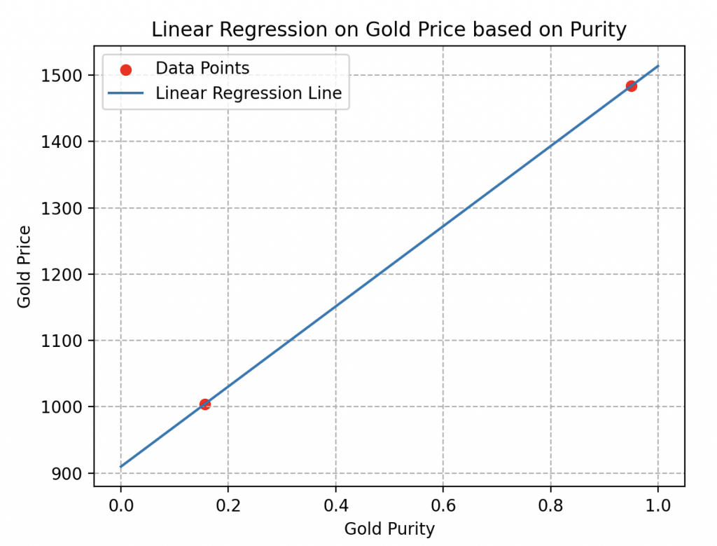
When indicated, this table constitutes a learning database. Each sample k is characterized by two elements: its purity \(x^{(k)}\) which varies between 0 (not gold) and 1 (pure gold), and its price \(y^{(k)}\) (which can range from 0 to infinity).

The collection of these samples represents a crucial moment in the life of this robotic scholar. Here are two essential aspects that it must take into consideration to make accurate estimates.

Large number of data: Wall-E quickly realizes that to obtain reliable estimates, he must have a large number of samples in his database.

Indeed, if we only consider two samples, as illustrated here, it is impossible to determine whether the price behavior is linear or not.

Many estimation curves could pass through these two points without reflecting reality. Like the two curves below, for example.

Data Diversity: another crucial detail to consider during the harvest is the variety of data.

Suppose Wall-E only considers pure samples or samples with extremely close purity (see the figure opposite).

In this situation, all samples will have almost the same price, preventing him from estimating the price of other gold alloys.

Conclusion of the Harvest: It is, therefore, imperative to gather a multitude of randomly chosen samples to avoid these limitations and ensure obtaining accurate estimates for a wide range of gold alloys.

Creation of the Linear Model

From these data, Wall-E develops what we have called a linear model \(f(x)=ax+b\) where aa and bb are the parameters of the model. An effective model minimizes the differences between Wall-E’s predictions \(f(x)\) and the actual values yy of the samples. Like a kind of modern gold prospector, Wall-E adjusts these parameters to best align his estimates with reality, creating an equation that subtly connects purity and the value of gold. Here is his initial attempt, which is not incredible at all.

Measuring Gold Treasures: The Cost Function

The next step in Wall-E’s learning process is to evaluate the performance of this model, meaning measuring the errors between its predictions and the values in the dataset.

For the small robot, the procedure is simple: each estimation, denoted k, in the dataset is compared to reality. Depending on the chosen approach, Wall-E’s program returns the corresponding error for each prediction, which we will denote as \(err(k)\).

Each of Wall-E’s estimations is thus associated with its own margin of error. Over iterations, these errors accumulate in number until reaching the total number of examples n in the dataset.

Therefore, all these errors are gathered in a function called the Cost Function, denoted \(Γ(a, b)\). It is a function depending on the parameters to be adjusted and simply calculates the average of all errors. Therefore, it is written as follows:

\begin{align*}\Gamma(a, b) &=\frac{err(1)+err(2)+\cdots+err(n)}{n}=\frac{1}{n}\sum_{k=1}^n err(k)\end{align*}

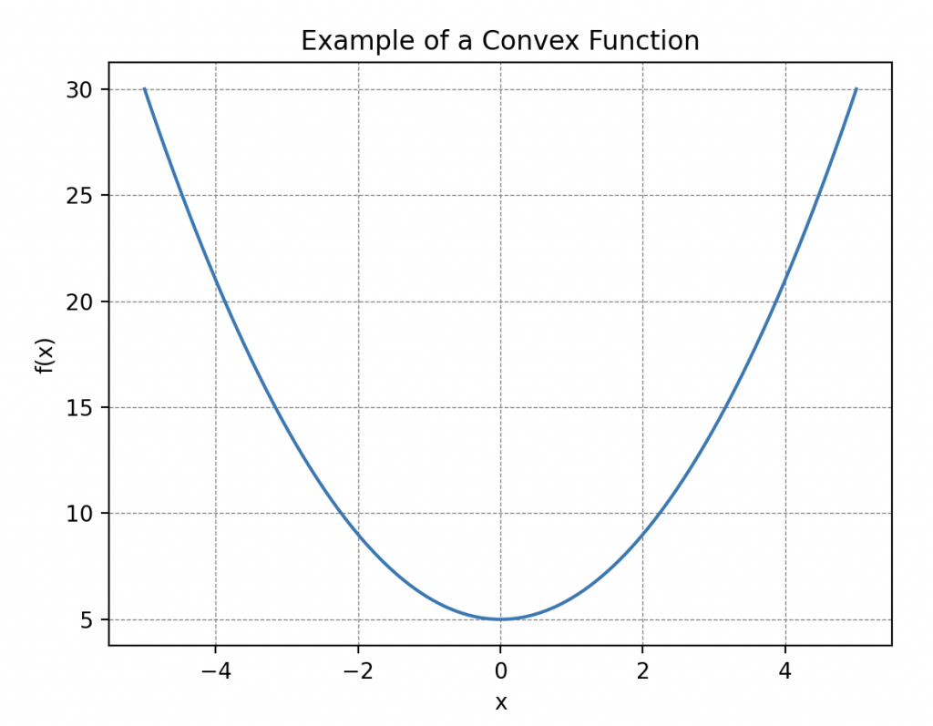
An important property to consider about this function is its convexity, meaning that its curve ‘faces upward everywhere.’ More precisely, this means that if you draw a line between two points on the curve, it always stays above or at the same level as the curve. Such curves always have a global minimum! This will be useful to us later.

However, what is error? How can it be defined? Before addressing these questions, it is crucial to discuss a mathematical concept: distance, which allows quantifying the separation between two given points.

Distances Explained by Hal

Wall-E, in the midst of contemplation, sought to understand why he needed to pay attention to the concept of distance. Perplexity engulfed him as he observed Hal, his loyal companion cockroach, sneak silently through the corners of the laboratory.

What could this meticulous and methodical exploration of space by Hal possibly signify?

He was far from imagining that behind these silent and discreet movements, Hal was, in his own way, sharing the subtleties of distances. Each maneuver between the objects in the room illustrated an essential mathematical rule. They counted up to four.

Positivity. In this choreography, Hal demonstrated the first rule: the positivity of distances. Explaining in his own way that the distance between his favorite hiding spot and the waste pantry was always positive, a fact simply illustrated by his trajectory (a length is not negative).

Wall-E, being a good scientist, expressed it in mathematical terms: The distance between any two points A and B must be positive or zero. This is written as,
\begin{align*}
\forall A, B \in E, \quad d(A,B)\geq 0.
\end{align*}

This symbol \(“\forall”\) means “for all” and \(“\in”\) means “in”. It reads, for all arbitrary elements A and B (here we are talking about points) in E, the distance between A and B is positive or zero.

Symmetry. The concept of symmetry was then highlighted by Hal, demonstrating how his movements from point A to point B were always identical, whether he went from B to A or from A to B. His subtle back-and-forth marked the idea of symmetry in this dance between points.

The little robot introduced this idea into his circuits: The distance between A and B must be the same as between B and A. Mathematically,
\begin{align*}
\forall A, B \in E, \quad d(A,B)=d(B,A).
\end{align*}

Separation. However, the most surprising demonstration for Wall-E was that of separation. Hal went to fetch two seeds that he placed in two different locations in the room. He then began a frenetic dance, leaving one seed fixed and bringing the other one back to it by performing a series of quick back-and-forths until finally sticking the two seeds together.

In this way, he wanted to illustrate to Wall-E that if the distance between these two points was zero, then the two points coincide. An impressive and clear representation of the separation rule.

He understood the lesson, which he translated into his own language: If the distance between A and B is zero, then A and B coincide.

\begin{align*}\forall A, B \in E, \quad d(A,B)=0 ⇒A=B.\end{align*}

This symbol “⇒” means “imply”.

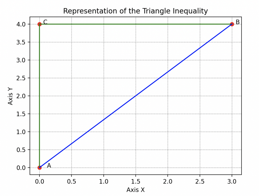
The Triangle Inequality. However, Hal’s lesson did not stop there as there was still another essential rule to analyze. He continued his exploration by illustrating the triangle inequality.

By moving between his hiding spot, Wall-E, and the pantry, Hal showed that the distance between his hiding spot and Wall-E is always less than the distance between his hiding spot and the pantry plus the distance between the pantry and Wall-E. This clever trick, teaching that the shortest path between two points is a straight line, captivated Wall-E.

He hastened to transcribe it all: If I take three points A, B, and C that do not coincide, then the distance between A and B is always less than or equal to the distance between A and C plus the distance between C and B.

\begin{align*}
\forall A, B, C \in E, \quad d(A,B)\leq d(A,C)+d(C,B).
\end{align*}

Thanks to Hal, Wall-E grasped that formally, a distance is a function that compares two points in a given space by assigning a non-negative real number, expressing the “length” between these two points, and follows specific rules.

This space can be the familiar two-dimensional plane as demonstrated by the cockroach or our three-dimensional space, or even much more exotic spaces.

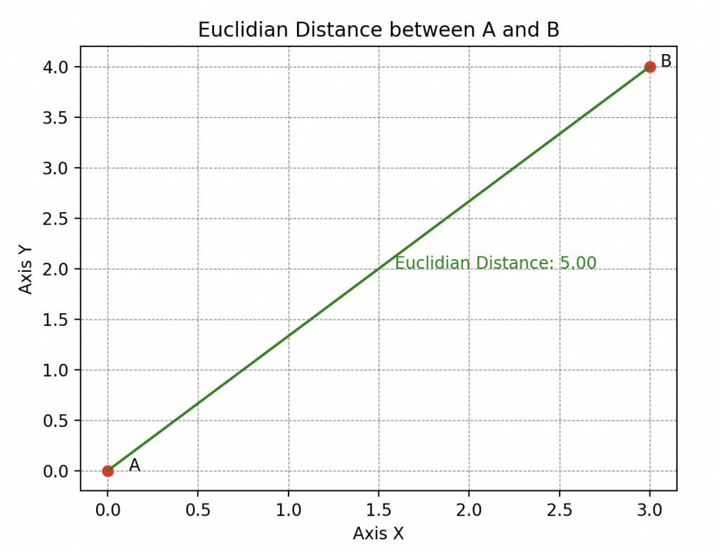
His abstraction skills also allow him to understand that there are different types of distances, among which the most well-known is the Euclidean distance (also called the 2-distance).

or the l’\(\infty\)-distance (also called the infinity-distance), which assesses the maximum distance between these points along any dimension.

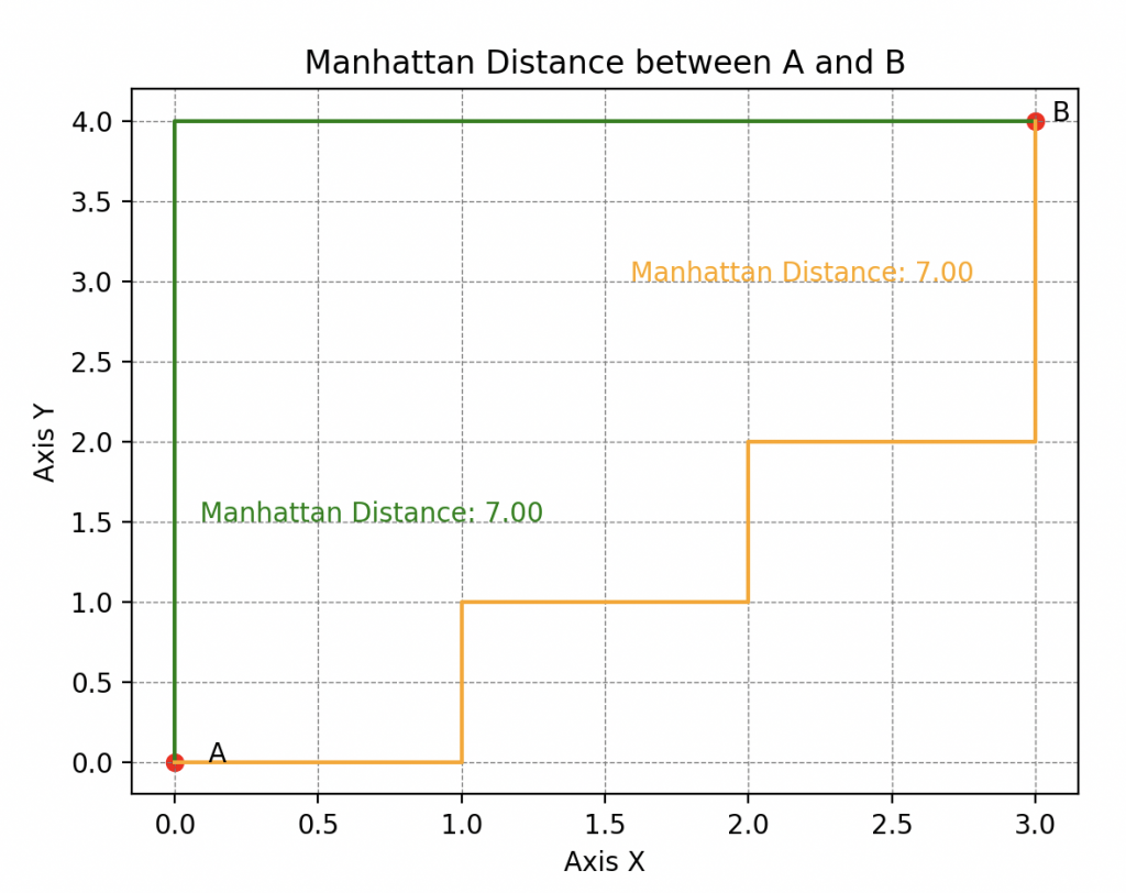
However, there is also the Manhattan distance (or 1-distance for purists), named so because it reflects the distance a taxi would have to travel in a network of streets forming orthogonal grids (typical of the street layout in Manhattan, hence the name).

We will explore these intricacies in detail in an upcoming article.

A Fatal Error

Now, why delve into the concept of distance in the context of evaluating Wall-E’s predictions? In fact, this leads us to consider what errors truly represent between the predictions and the actual values in the dataset.

Imagine that Wall-E evaluates the first sample, a one-kilogram gold alloy with a purity of 0.72 and an actual price of 1231 bolts, but predicts 1331 bolts. You observe a difference of -130 bolts. Here, we obtain a negative value, but in another example, it could be positive. This duality between positive and negative values is not practical.

To solve this problem, two options are available to us:

• The first option is to consider the absolute value of each difference (remove the minus sign when present). The error obtained is called the absolute error, denoted AE.

In the previous example, we would have \(AE(1) = | 1231–1331| = |-130|=130\).

• The second option is to calculate the square of each difference. This error is called the squared error, noted SE.

Here, we would have a squared error \(SE(1)= (1231–1331)^2=(-130)^2=16900\).

We notice that the second option greatly amplifies the errors, but we will see how to balance these differences later.

Thus, by applying either of these options, we choose how we want to measure errors, i.e., a distance. The \(\infty\)-distance for the first or the Euclidean distance for the second.

Now, the procedure is simple: each estimate, denoted by k, in the Dataset is compared to reality. Depending on the chosen approach, Wall-E’s program returns the corresponding error. Moreover, depending on the chosen distance, the cost function is named differently:

• If we consider the approach of absolute errors, it is called the Mean Absolute Error, denoted MAE, and is written as:

\begin{align*} MAE(a, b) &=\frac{AE(1)+AE(2)+\cdots+AE(n)}{n}=\frac{1}{n}\sum_{k=1}^n AE(k)\\ &= \frac{1}{n}\sum_{k=1}^n\left|f\left(x^{(k)}\right) – y^{(k)}\right|=\frac{1}{n} \sum_{k=1}^{n} \left|ax^{(k)} + b- y^{(k)}\right|. \end{align*}

• While the approach of squared errors provides us with a cost function called Mean Squared Error, denoted MSE, and is written as:
\begin{align*}
MSE(a, b) &=\frac{SE(1)+SE(2)+\cdots+SE(n)}{n}=\frac{1}{n}\sum_{k=1}^n SE(k)\\
&= \frac{1}{n}\sum_{k=1}^n\left(f\left(x^{(k)}\right) – y^{(k)}\right)^2=\frac{1}{n} \sum_{k=1}^{n} \left(ax^{(k)} + b- y^{(k)}\right)^2.
\end{align*}

To rescale the errors calculated by this function, we simply take its square root. The function obtained in this way is called the Root Mean Squared Error, noted RMSE.

Here’s an example to illustrate the calculation where Wall-E estimates the value of only five samples (with five differences).

Differences	-100	7	-2	42	13
Errors AE	100	7	2	42	13
Errors SE	10 000	49	4	1764	169

Calculation of MAE

Calculation of RMSE

\begin{align*}MAE(a, b) =\frac{100 + 7 + 2 + 42 + 13}{5} = 32.8.\end{align*}

\begin{align*}RMSE(a, b) =\sqrt{\frac{10000 + 49 + 4 + 1764 + 169}{5} }= 48.96.\end{align*}

Why choose one or the other? To answer this question, let’s introduce Eve.

In addition to her ability to distinguish organic objects, she has a sophisticated self-defense system. She has been trained to estimate the distance (in centimeters) between the impact of her shots and the center of the target. Eve trains two models to find the one that will minimize errors.

	Error 1	Error 2	Error 3	Error 4	MAE
Model 1	20	0	0	0	5
Model 2	6	5	6	4	5.25

	Error 1	Error 2	Error 3	Error 4	RMSE
Model 1	20	0	0	0	10
Model 2	6	5	6	4	5.31

Here we observe that the MAE of model 1 is smaller than that of model 2, so Eve will choose model 1 to estimate her shots.

However, in the first model, we can see that Eve makes almost no errors except for her first shot where she is off by 20 cm.

This is a non-negligible and dangerous quantity, as it could cause harm to someone if her arsenal is not precise enough.

In this table, it’s completely different; we observe that the RMSE of model 1 is much worse than model 2 as it shows a much larger error.

Eve would tend to choose model 2 in this case. In fact, RMSE penalizes large errors much more than MAE.

If Eve favors Mean Absolute Error (MAE), it means she wants to minimize the absolute differences between the impact of her shots and the target. This suggests that for Eve, each difference has the same importance. A difference of 20 units is considered twenty times more important than a difference of 1 unit.

On the other hand, if Eve chooses to favor Root Mean Squared Error (RMSE), it means she wants to emphasize large differences. In this case, more significant errors have a more significant weight. Indeed, a difference of 20 units is 400 times more important than a difference of one unit. So, if Eve wants to eliminate shots with very large differences, the model based on RMSE would be more suitable.

These choices of cost functions depend on Eve’s goals: if she wants to reduce large differences, she will favor MSE. On the other hand, if she wants a balanced assessment of all differences, she will opt for MAE. Also, there are other ways to measure errors, but we won’t discuss them here.

A Small Step for the Robot, a Giant Leap for the Algorithm

What Wall-E enjoys most is learning by himself which parameters minimize the cost function, that is, the parameters that give us the best possible model. To find these optimal parameters, Wall-E uses a well-known optimization algorithm called gradient descent. Imagine this step as if Wall-E is meticulously adjusting the knobs of his mathematical model to reach the level of expertise needed in predicting the price of gold based on its purity.

Let's Descend!

The concept of gradient descent is simple: envision Wall-E lost on the slopes of a waste mountain in thick fog, recycling what’s left for him to do. Unfortunately for him, his batteries are dangerously fading, so he must reach his small spaceship located at the lowest point, but he can only see the immediate slopes around him. Thus, at each step of length \(\delta\) (that’s the Greek letter delta), he chooses the direction that makes him descend as quickly as possible. As he advances, he adjusts his direction based on the slopes he perceives, gradually approaching the lowest point.

Of course, the choice of the value \(\delta\) is crucial in gradient descent. Because imagine if Wall-E takes steps that are too small, he will take too long to reach the bottom, or if he uses his jetpack to fly over very large distances, he might overshoot his refuge.

Let’s go back to our initial problem. The mountain of waste symbolizes our cost function, Wall-E’s position parameters on the mountain represent the parameters of our linear regression model, and the steps translate what is called Wall-E’s learning rate. So, breaking down Wall-E’s actions algorithmically, we have:

• Our robot calculates the gradients, meaning the slope along the two axes (a and b) of the cost function at each iteration. Mathematically, this involves calculating these two quantities:

\begin{align*} \frac{\partial \Gamma(a, b)}{\partial a}\quad\text{et}\quad \frac{\partial \Gamma(a, b)}{\partial b} \end{align*} Mathematicians will have understood it well; this is nothing more than the calculation of the derivative of a function with several variables.

• He updates the parameters, bringing him closer and closer to the minimum of the cost function. The updated parameters are referred to as \(a^*\) and \(b^*\) and write \begin{align*} a^*&=a-\delta\times\frac{\partial \Gamma(a, b)}{\partial a}\\ b^*&=b- \delta\times\frac{\partial \Gamma(a, b)}{\partial b} \end{align*} Thus, the new parameters are simply defined as the old position minus the learning rate \(\delta\) multiplied by the value of the slope. By analogy, it’s Wall-E’s position after taking a step in the direction where the slope is the steepest.

• He restarts until he finds the minimum of the cost function.

It’s important to understand that gradient descent is an iterative process, meaning it repeats many times until Wall-E reaches a point where the cost function is minimal, and its predictions are as accurate as possible.

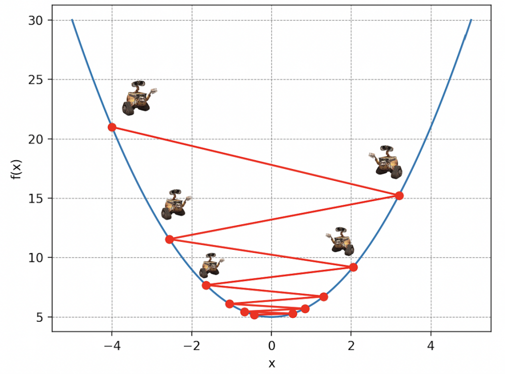
Regarding the learning rate, some details need to be clarified. As in the previous metaphor, the choice of the value of \(\delta\) is crucial.

A too small \(\delta\) could slow down convergence because parameter adjustments would be tiny at each step, while a too large \(\delta\) could lead to oscillations or even prevent convergence, as adjustments might overshoot the desired minimum. Therefore, choosing the value of \(\delta\) is therefore crucial for Wall-E’s algorithm to converge efficiently towards the optimal solution.

When will we arrive ?

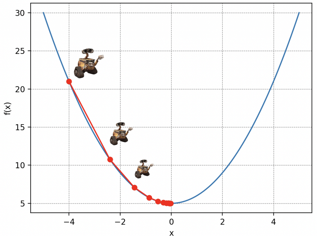
It’s been a little while now that our brave robot has been moving desperately in the dark, blinded by Mother Nature. He wonders when he will reach the bottom of the mountain. Just like in this situation, in machine learning, reaching the minimum of the cost function – the equivalent of shelter for Wall-E – can seem tricky. His position is uncertain, and to get there, Wall-E must adjust his progress, taking into account the length of his steps and the number of these steps.

To navigate, Wall-E must meticulously record each of his positions along the mountain’s slope, which is called the descent story. By keeping an accurate record of each step, he can then plot his trajectory, creating a “descent curve.” This allows him to visualize his path, measure his progress, and determine if he is close to the lowest point. Below is an example, assuming Wall-E is randomly placed on the mountain.

In the field of Machine Learning, the descent story is actually called the cost history as it provides the values of the cost function based on key variables such as the learning rate and the number of iterations of the gradient descent algorithm.

Moreover, its graphical representation, referred to as the descent curve, is actually called the learning curve. It is essential for assessing the performance of a model because it dynamically illustrates the evolution of the model’s accuracy.

In this particular case, after about ten steps, Wall-E seems to stop descending further, indicating that it has reached its shelter. The additional 40 steps are therefore unnecessary. This information is crucial in computer science, as it allows us to avoid running the algorithm unnecessarily, potentially saving time and resources, especially when certain simulations can take considerable time, ranging from days to weeks.

In its Printed Circuits: Estimating the Price of Gold

But what exactly is happening in the electronic brain of our adorable robot? Before performing any addition, Wall-E translates not only the entire dataset into a table but also the model parameters and gradients: a kind of encrypted language for machines known as matrix form that greatly simplifies calculations. More precisely, this gives rise to a vector. \(\mathbf{Y}\) composed of n elements corresponding to the prices of the n gold samples,

\begin{equation*} \mathbf{Y}=\begin{bmatrix} y^{(1)} \\ y^{(2)} \\ \vdots\\ y^{(n)} \end{bmatrix} \end{equation*}

accompanied by a matrix \(\mathbf{X}\) with n rows and \(m+1\) columns that accurately encapsulates each of the m features (in this case, there is only one \(m=1\)) and a column containing only 1s, which we’ll call the “bias.”

\begin{equation*} \mathbf{X}=\left[ \begin{array}{cc} x^{(1)} & 1\\ x^{(2)} & 1\\ \vdots & \vdots\\ x^{(n)} & 1 \end{array} \right]. \end{equation*}

This last one simply allows us to perform the necessary matrix calculations for learning. It’s worth noting that, in general, we have

\begin{equation*} \mathbf{X}=\left[ \begin{array}{cccc} x^{(1)}_1 & \cdots & x^{(1)}_m & 1\\ \vdots & \ddots & \vdots & \vdots \\ x^{(n)}_1 & \cdots & x^{(n)}_m & 1 \end{array} \right]. \end{equation*}

Simultaneously, a vector called “parameter” \(\mathbf{P}\) (a column) makes its entrance, carefully bringing together all the parameters of our model, namely a and b.

\begin{equation*} \mathbf{P}=\begin{bmatrix} a \\ b \end{bmatrix}. \end{equation*}

Don’t forget that we are looking for \(\mathbf{P}\) such that it minimizes the cost function. Thanks to this, Wall-E can express all the learning steps easily and estimate the price of a gold nugget with an unknown value:

• The Harvest is carried out by displaying the data in a matrix: each sample, with its purity and price characteristics, finds its place in this matrix.

• The Model Creation is the process where Wall-E defines the parameters shown in the column \(\mathbf{P}\) chosen randomly, which are used to establish the linear relationship between the purity and the price of gold. \(\mathbf{F(\mathbf{X})}=\mathbf{X\times P}\).

• The Cost Function is redefined as follows: \begin{align*} \Gamma(\mathbf{P})=\frac{1}{n}\left(\mathbf{F(X)-y}\right)\cdot\left(\mathbf{F(X)-y}\right) \end{align*} where \(\cdot\) denotes the dot product (we will talk about the scalar product in another article).

• Finding the Minimum involves calculating the gradient: \begin{align*}\frac{\partial }{\partial \mathbf{P}} \Gamma(\mathbf{P})=\frac{1}{n}\mathbf{X\cdot\left(F(X)-y\right)}\end{align*} and iteratively applying gradient descent to update the parameter P: \begin{align*}\mathbf{P^*}=\mathbf{P}-\delta \frac{\partial }{\partial \mathbf{P}}\Gamma(\mathbf{P})\end{align*} where \(\mathbf{P^*}\) is the new parameter.

Wall-E, by carefully applying all the steps, is now ready to estimate the price of gold based on the purity you provide! Here is the final curve he obtains.

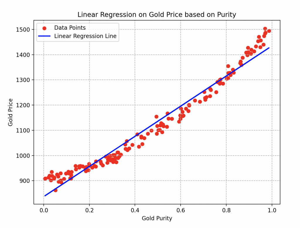
The parameters a and b of the blue line are respectively equal to 493.56 and 886.18. For the gradient descent, he used a learning rate of 0.2 and performed about twenty iterations of the algorithm.

It can be easily observed that by choosing a gold alloy with a purity of 0.6, its estimated price would be around 1200 bolts.

Knowledge Transfer and Model Performance: Lessons Applicable to All Regressions

All the steps and calculations performed to estimate the price of gold based on its purity through linear regression are fundamentally similar to those carried out for nonlinear regression or other types of machine learning models!

Wall-E, the little robot passionate about estimating the price of gold, follows a well-defined sequence to train its model, minimize error, and adjust parameters to predict the price of gold based on its purity. The process involves transforming data into matrices, creating the model, defining the cost function to evaluate errors, minimizing this function by iteratively adjusting parameters, and finally obtaining the optimal parameter to accurately estimate the price of gold.

This process is flexible and can be applied to different situations and types of learning models, thus adapting to more complex problems requiring more sophisticated models. Wall-E’s success in estimating the price of gold demonstrates the power and efficiency of these methods, paving the way for broader and more diverse applications of machine learning in various contexts.

But there is still one last thing to consider: The Coefficient of Determination, also known as \(R^2\). It plays a crucial role in evaluating Wall-E’s model performance as it measures how well the model fits the data compared to the variations in it. In mathematical terms, it is written as follows:

\begin{equation}R^2 = 1 – \frac{\sum_{k=1}^{n} \left(y^{(k)}- f(x^{(k)})\right)^2}{\sum_{k=1}^{n} (y^{(k)}- \bar{y})^2}\end{equation}

where \(\bar{y}\) is nothing but the average of our sample values (in our case, it is simply the mean price). Despite its seemingly complex appearance, it conceals a simple fraction to understand. By rewriting it in a more digestible form, we have,

\begin{equation}R^2 = 1 – \frac{Errors}{Variance}.\end{equation}

Remember (see the article “Beating the Game Master“) that variance is a measure of the dispersion of sample values.

So, for Wall-E, getting an \(R^2\) close to 1 would be ideal, implying that the right fraction is close to 0. This means that errors are largely negligible compared to how the data disperses, and the model proposed by Wall-E fits well with the sample values.

On the contrary, if \(R^2\) is close to 0, it would indicate that the model does not explain the data variability well, and predictions may be less reliable because errors are of the same order of magnitude as the variance.

With all these explanations, Wall-E embarked on calculating the coefficient of determination \(R^2\) to assess the quality of his previous model.

The result is quite gratifying, with a commendable score of 0.93. In other words, the model fits remarkably well with the data, covering approximately 93% of the observed variability.

This performance confirms the effectiveness of his approach in estimating the price of gold based on its purity!

However, Wall-E, as an tireless perfectionist, is not content with already achieved success. He is constantly seeking ways to improve his model.

Thus, he decides to transcend the initial linear model by opting for a polynomial approach (of degree 2). He modifies the reference function to \(f(x) = ax^2 + bx + c\) and meticulously repeats all the steps of the algorithm, leaving nothing to chance. Here are the results he obtained.

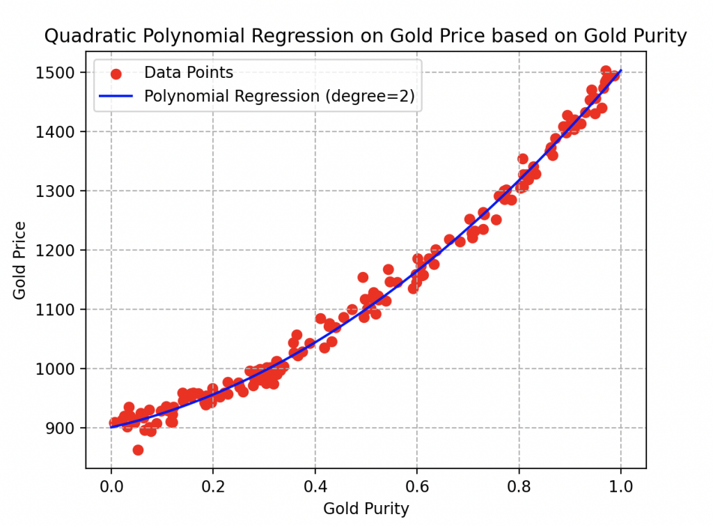
The curve fits the data really well, and for good reason. With parameters values of 273.84, 404.43, and 837.08, he achieves an outstanding coefficient of determination of 97%!

Observe here that a gold sample with a purity of 0.6 would be worth around 1160 bolts.

In contemplating this success, one cannot help but eagerly anticipate Wall-E’s future explorations in the complex world of modeling and machine learning.

Successful Exploration of the Intricacies of Regression: Next Step, the Fascinating World of Classification

In this captivating exploration of regression problems, we delved into the fascinating universe of mathematical modeling, with Wall-E as our intrepid guide. From gradient descents to learning curves, and through the definition of errors, we demystified key aspects of regression, unveiling the underlying magic of Machine Learning.

As we let Wall-E rest his circuits after his regression exploits, get ready to embark on a new adventure in our upcoming article. We’ll delve into the mysteries of classification problems, exploring how models can learn to categorize and make decisions in a world of complex data. Stay tuned for an even deeper dive into the dynamic universe of machine learning with Wall-E as your faithful travel companion!

Bibliography

G. James, D. Witten, T. Hastie et R. Tibshirani, An Introduction to Statistical Learning, Springer Verlag, coll. « Springer Texts in Statistics », 2013

D. MacKay, Information Theory, Inference, and Learning Algorithms, Cambridge University Press, 2003

T. Mitchell, Machine Learning, 1997

F. Galton, Kinship and Correlation (reprinted 1989), Statistical Science, Institute of Mathematical Statistics, vol. 4, no 2,‎ 1989, p. 80–86

C. Bishop, Pattern Recognition And Machine Learning, Springer, 2006

G. Saint-Cirgue, Machine Learnia, Youtube Channel

D.V. Lindley, Regression and correlation analysis, 1987

Non-Optimal Linear Regression


import numpy as np
import matplotlib.pyplot as plt
from sklearn.linear_model import LinearRegression

# Parameters of the quadratic function
a = 400
b = 200
c = 900

# Generate 150 points between -100 and 100
np.random.seed(42)

X = np.random.uniform(0, 1, 150)

# Create Y values based on the quadratic function with Gaussian noise

Y = a * X**2 + b * X + c + np.random.normal(0, 15, 150)

# Reshape the data for modeling
X = X.reshape(-1, 1)
Y = Y.reshape(-1, 1)

# Perform linear regression
model = LinearRegression()
model.fit(X, Y)

# Display the data
plt.figure(figsize=(8, 6))
plt.scatter(X, Y, color='red',label='Data Points')
plt.plot(X, 500 * X +  c, color='blue', linewidth=2, label='Linear Regression Line')
#plt.plot(X, model.predict(X), color='blue', linewidth=2, label='Linear Regression Line')
plt.title('Linear Regression on Gold Price based on Purity')
plt.xlabel('Gold Purity')
plt.ylabel('Gold Price')
plt.legend()
plt.grid(ls='--')
plt.show()

Optimal Linear Regression with Learning Curve


import numpy as np
import matplotlib.pyplot as plt

# Parameters of the quadratic function
a = 400
b = 200
c = 900

# Generate random data
np.random.seed(42)
x = np.random.uniform(0, 1, 150)
y = a * x**2 + b * x + c + np.random.normal(0, 15, 150)
y = y.reshape(y.shape[0], 1)  # Reshaping y to fit the required shape

# Create the feature matrix X
X = np.vstack((x, np.ones(len(x)))).T

# Initialize the theta parameters for the linear model
theta = np.random.randn(2, 1)

# Define the linear model function
def model(X, theta):
    return X.dot(theta)

# Define the cost function
def cost_function(X, y, theta):
    m = len(y)
    return 1 / (2 * m) * np.sum((model(X, theta) - y)**2)

# Define the gradient calculation function
def grad(X, y, theta):
    m = len(y)
    return 1 / m * X.T.dot(model(X, theta) - y)

# Define the gradient descent function
def gradient_descent(X, y, theta, learning_rate, n_iterations):
    cost_history = np.zeros(n_iterations)
    for i in range(n_iterations):
        theta = theta - learning_rate * grad(X, y, theta)
        cost_history[i] = cost_function(X, y, theta)
    return theta, cost_history

# Define the learning rate and number of iterations
learning_rate = 0.2
n_iterations = 20

# Perform gradient descent to optimize the parameters
theta_final, cost_history = gradient_descent(X, y, theta, learning_rate, n_iterations)

# Make predictions with the optimized parameters
predictions = model(X, theta_final)

# Plot the data points and the linear model predictions
plt.scatter(x, y, c='r',label='Data Points')
plt.plot(x, predictions, c='blue',label='Linear Regression Line')
plt.xlabel('Gold Purity')
plt.ylabel('Gold Price')
plt.title('Linear Regression on Gold Price and Gold Purity')
plt.legend()
plt.grid(ls='--')
plt.show()

# Plot the cost history during gradient descent
plt.plot(range(n_iterations), cost_history)
plt.xlabel('Number of Steps')
plt.ylabel('Descent')
plt.title('Descent History during Gradient Descent')
plt.grid(ls='--')
plt.show()

# Calculate the coefficient of determination (R-squared)
def coef_determination(y, pred):
    u = ((y - pred)**2).sum()
    v = ((y - y.mean())**2).sum()
    return 1 - u / v

# Print Final theta

print(theta_final)

# Print the R-squared value
print(coef_determination(y, predictions))

# Display the first 5 samples of the data
print("First 5 samples of the data:")
for i in range(5):
    print(f"Sample {i + 1} - Gold Purity: {x[i]:.4f}, Gold Price: {y[i][0]:.4f}")

Polynomial Regression


import numpy as np
import matplotlib.pyplot as plt

# Parameters of the quadratic function
a = 400
b = 200
c = 900

# Generate random data
np.random.seed(42)
x = np.random.uniform(0, 1, 150)
y = a * x**2 + b * x + c + np.random.normal(0, 15, 150)
y = y.reshape(y.shape[0], 1)  # Reshaping y to fit the required shape

# Create the feature matrix X

X = np.vstack((x**2,x, np.ones(len(x)))).T


print(X.shape)

# Initialize the theta parameters for the linear model
theta = np.random.randn(3, 1)

# Define the polynomial model function
def model(X, theta):
    return X.dot(theta)

# Define the cost function
def cost_function(X, y, theta):
    m = len(y)
    return 1 / (2 * m) * np.sum((model(X, theta) - y)**2)

# Define the gradient calculation function
def grad(X, y, theta):
    m = len(y)
    return 1 / m * X.T.dot(model(X, theta) - y)

# Define the gradient descent function
def gradient_descent(X, y, theta, learning_rate, n_iterations):
    cost_history = np.zeros(n_iterations)
    for i in range(n_iterations):
        theta = theta - learning_rate * grad(X, y, theta)
        cost_history[i] = cost_function(X, y, theta)
    return theta, cost_history

# Define the learning rate and number of iterations
learning_rate = 0.2
n_iterations = 20

# Perform gradient descent to optimize the parameters
theta_final, cost_history = gradient_descent(X, y, theta, learning_rate, n_iterations)

# Make predictions with the optimized parameters
predictions = model(X, theta_final)


# Plot the data points and the polynomial regression predictions
plt.scatter(x, y, c='r', label='Data Points')
plt.plot(x, predictions, c='blue', label='Polynomial Regression Line')
plt.xlabel('Gold Purity')
plt.ylabel('Gold Price')
plt.title('Polynomial Regression on Gold Price and Gold Purity')
plt.legend()
plt.grid(ls='--')
plt.show()

# Plot the cost history during gradient descent
plt.plot(range(n_iterations), cost_history)
plt.xlabel('Number of Steps')
plt.ylabel('Descent')
plt.title('Descent History during Gradient Descent')
plt.grid(ls='--')
plt.show()


# Calculate the coefficient of determination (R-squared)
def coef_determination(y, pred):
    u = ((y - pred)**2).sum()
    v = ((y - y.mean())**2).sum()
    return 1 - u / v

# Print Final theta
print(theta_final)

# Print the R-squared value
print(coef_determination(y, predictions))

Immerse yourself in our universe