
Waste Allocation Load Lifter: Earth Class
Episode III
By Jordan Moles on December 2, 2023

As a robot faithful to its mission and amidst occasional gold estimations, Wall-E does not forget its primary task: sorting waste. It is during its expeditions to remote locations on the planet that it encounters the ultimate challenge that stimulates its curious mind. Among the objects it gathers, Wall-E comes across a diverse collection of old electronic components—some in good condition that it brings back to the base, and others defective that it stores in a corner.
Passionate about such objects, it begins to unscrew, pull apart, and carefully categorize each component into two distinct categories (binary classification): on one side, the precious metal pieces that it will sort later (multiclass classification), and on the other, the worthless plastic. The fundamental question is: how does it accomplish such a mission?
It is strongly recommended to have read episodes I and II before continuing!
Wall-E's New Horizons: The Classification
The epic journey of our intrepid lone robot, Wall-E, takes on a fascinating new dimension as he explores the vast realm of classification. After brilliantly mastering the art of regression in the previous episode (see the article “Wall-E: The Little Gold Miner“), Wall-E courageously embarks on a new phase by delving into binary classification between precious metals and plastics. This initial preparatory step marks the beginning of a more complex quest, where Wall-E boldly deploys his classification skills to navigate through the diverse metals that line his path.
Building on his initial successes, Wall-E decides to broaden his scope by tackling the multi-class classification of metals, making the K-Nearest Neighbors (KNN) algorithm his preferred ally. This new challenge requires Wall-E to gain a deeper understanding, as he must not only distinguish between two categories but also classify different types of metals such as bronze, gold, and silver.
This new phase of his adventure marks Wall-E’s transformation towards broader and more sophisticated classification horizons. Each step of this exploration adds a new dimension to his skills, preparing Wall-E to face more complex challenges than simple binary sorting. In this endeavor, model selection proves crucial to ensure the accuracy of his predictions. Wall-E apprehends the importance of the cross-validation process and meticulously explores the nuances of hyperparameter tuning, thereby ensuring the robustness and efficiency of his model.
The Key Element: Always the Data
In his exploration to decipher the nature of electronic components, Wall-E draws upon the information stored during his learning experiences with his creators. This approach aims to build an extensive and diverse set of samples, running in parallel with his challenges related to regression.
Meeting the Samples
Each example \(k\) was an element with specific characteristics, such as density \(x^{(k)}\), thermal conductivity \(x_2^{(k)}\), electrical conductivity \(x_3^{(k)}\), etc. To illustrate our case simply, we will consider only the density variable \(x^{(k)}\) for now.
Thus, for each sample \(k\), Wall-E notes whether it is a metal (labeled as \(y^{(k)}=1\)) or plastic (labeled as \(y^{(k)}=0\)). These samples and their labels form his training dataset. Here is a concrete example of 5 samples (among the 650 he already knows).
| Density | Type of Component | |
|---|---|---|
| Sample 1 | 2.165747 | Plastic |
| Sample 2 | 7.151579 | Metal |
| Sample 3 | 0.901240 | Plastic |
| Sample 4 | 19.24357 | Metal |
| Sample 5 | 12.54564 | Metal |
The Decision Boundaries
The difference with the previous problem is that here we need to define what we call a decision boundary. Let’s explain this concept simply. Instead of looking at each object individually, Wall-E decides to divide this space into different regions. Each region would be intended to receive a specific type of object, either metal or plastic. The boundaries of these regions will define decision boundaries, and that’s where the heart of the classification problem lies.
When Wall-E draws these boundaries, he wants to ensure that similar objects are in the same region. This means that objects close to each other in density tend to have the same label, either metal or plastic. Ideally, he would like these two groups to be perfectly separated, as if they were in distinct boxes. A simple line could do the trick.
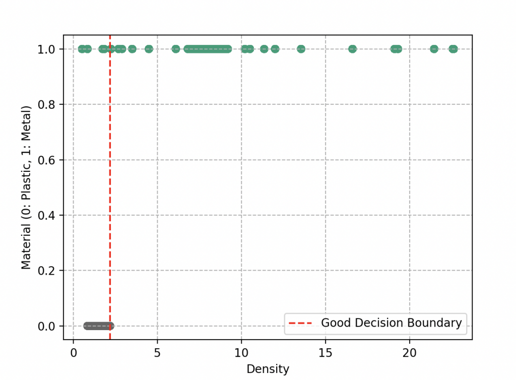

However, reality is not always so simple. Sometimes, there are objects that are misplaced and end up on the other side of the line. This is what happens in our example when some plastics have a higher density than some metals (such as rubber and lithium, which end up on the left side of the decision boundary). This poses a challenge for Wall-E. He must now judge his work based on the quality of the separation. The clearer the separation, the better. Misclassified objects are like errors on his sorting sheet, and as usual, he wants to minimize these errors.
Wall-E is also aware that he should not complicate things by drawing zigzagging and complex boundaries. These complicated boundaries might capture all objects, but it could also lead to overfitting, where each object is in its own region. This is called overfitting (we’ll see that in a few sections).
Creation of the Binary Classification Model
Driven by the desire to make sense of these electronic components, Wall-E embarks on the creation of a binary classification model. This model will take the features of a component as input and output a prediction of its nature. After exploring different approaches, including linear regression as he knows with the function \(f(x) = ax + b\) (with parameters a and b) that does not fit the data at all,


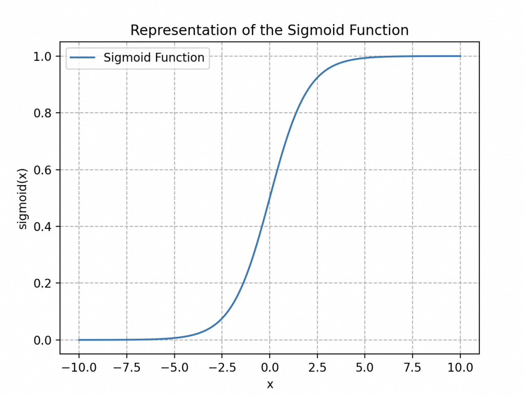
Wall-E opts instead for a classic Logistic Regression model, whose associated function (ranging between 0 and 1) is expressed as follows:
\begin{align*}
\sigma(x)=\frac{1}{1+\exp{(-x)}}
\end{align*}
It is called the logistic or sigmoid function (due to its “S”-shaped curve, see figure on the side).
By applying this function to our dataset, we obtain
\begin{align*}
\sigma(z)=\frac{1}{1+\exp{(-z)}}
\end{align*}
where \(z\) can be a linear function like \(ax + b\) or a polynomial function like \(ax^2 + bx + c\) (a polynomial of degree 2), with \(a\), \(b\), and \(c\) as parameters to be adjusted.
The significant advantage of such a function is that we can easily define a decision boundary by setting what is called a decision threshold value.


To formally understand why we introduce such a function, it is crucial to grasp that in the world of classification, Wall-E’s idea is to estimate the probability of an sample belonging to each category (metal or plastic). This allows confidently classifying each new observation into the category associated with the highest probability. Thus, when the estimation is close to the correct answer, the probability should be very close to 1, and conversely, if the estimation deviates from reality, the probability is almost zero.
The robot draws inspiration from this fundamental notion when he approaches the concept of the sigmoid function. He understands that this function can be used to transform the results of logistic regression into probabilities. As if applying a kind of mathematical filter to his evaluation, the sigmoid function assigns to each component a probability of belonging to a given category. Thus, if this probability is greater than 0.5, the object is classified in the “metal” category, and if it is less than 0.5, it is classified as plastic.
Prediction Evaluation: The Cost Function
Wall-E has developed his model, but he wants to evaluate the accuracy of his predictions. To do this, he undertakes to use one of the regression cost functions, the Mean Squared Error (MSE, see the article “Wall-E: The Little Gold Miner“), defined as follows:
\begin{align*}
MSE(a, b) =\frac{1}{n} \sum_{k=1}^{n} \left(\sigma(x^{(k)})- y^{(k)}\right)^2.
\end{align*}
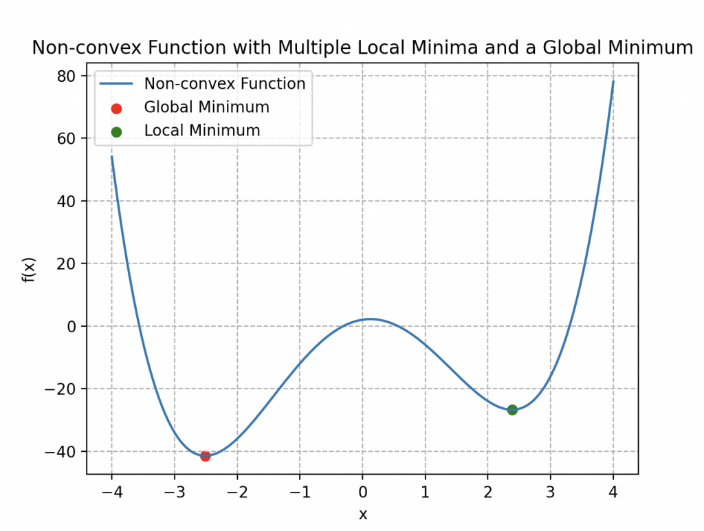
However, he finds himself facing a new significant challenge, as illustrated in the image on the side.
This cost function does not exhibit convexity; in fact, it has multiple local minima. This characteristic makes the gradient descent algorithm less effective because, using the analogy of a mountainous terrain, Wall-E might get trapped in a local minimum that is not necessarily the global minimum of the curve.
He introduces a new cost function using the logarithm:
\begin{align*}
L(a,b)=-\frac{1}{n}\sum_{k=1}^n\left[y^{(k)}\log{\left\{\sigma\left(ax^{(k)}+b\right)\right\}}+\left(1-y^{(k)}\right)\log{\left\{1-\sigma\left(ax^{(k)}+b\right)\right\}}\right]
\end{align*}
This complex cost function, although it may seem intimidating at first, is actually a powerful tool for evaluating the model’s performance. Let me delve deeper to explain why Wall-E chose this function and how it works.
The main goal of a cost function is to measure how well the model’s predictions match the actual values. The closer this match, the lower the value of the cost function. In the case of the first cost function, Wall-E had used a more direct approach, where he compared the model’s predictions (obtained by applying the sigmoid function to weighted inputs) to the true values. However, he noticed that this approach could pose problems during optimization.
The new cost function introduced by Wall-E uses the logarithm for a specific reason. It consists of two parts: one for cases where the class label is 1 (metal) and one for cases where the label is 0 (plastic). Let’s see in detail how these parts work.
The first part of the cost function, when a label is 1, is represented by the following term:
\begin{align*}
-y^{(k)}\log{\left\{\sigma\left(x^{(k)}\right)\right\}}
\end{align*}
Here, \(y^{(k)}\) is the true class value for training example \(k\), and \(x^{(k)}\) is the corresponding input. When \(y^{(k)}\) is 1 (the example belongs to the metal class), and the prediction \(\sigma\left(x^{(k)}\right)\) approaches 1, the value of \(-\log{\left\{\sigma\left(x^{(k)}\right)\right\}}\) tends toward 0, contributing to a low cost value for this example (the error is low because our prediction is good). On the other hand, if the prediction is close to 0, the value of \(-\log{\left\{\sigma\left(x^{(k)}\right)\right\}}\) becomes very large, leading to an increase in cost.

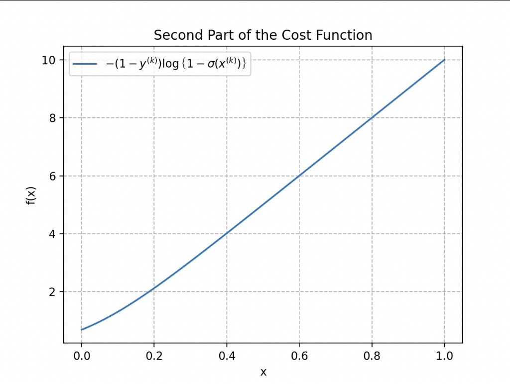
The second part of the cost function addresses cases where the label is 0:
\begin{align*}
-\left(1-y^{(k)}\right)\log{\left\{1-\sigma\left(x^{(k)}\right)\right\}}
\end{align*}
When \(y^{(k)}\) is 0 (the example belongs to the plastic class) and the prediction \(\sigma\left(x^{(k)}\right)\) is close to 0, the term \(\log{\left\{1-\sigma\left(x^{(k)}\right)\right\}}\) tends toward 0, contributing to a low cost. However, if the prediction approaches 1, \(\log{\left\{1-\sigma\left(x^{(k)}\right)\right\}}\) becomes large, increasing the cost.
Thus, when \(y^{(k)}\) is 1 in the cost function, only the first part of the function comes into play, and if it is 0, the other part is considered.
The total cost function is the average of these two parts, taken over the entire training set \(n\), to obtain an overall measure of the model’s fit to the training data. This allows evaluating the model’s prediction errors in a way that penalizes more significant errors.
Now, why choose such a complex cost function? The goal is to enable more efficient optimization of the model. This cost function has the advantage of possessing a convexity property, meaning it has only one global minimum and no local minima. This greatly facilitates the use of optimization algorithms such as gradient descent to adjust the model parameters. By avoiding local minima, Wall-E can be more confident that the optimization will lead to a higher-quality solution.
The Return of the Gradient Descent
Do you remember gradient descent for regression? We do exactly the same thing but with the new cost function. Algorithmically, we have:
• Our robot calculates the gradients of the cost function at each iteration, which can be expressed mathematically as follows:
\begin{align*}
\frac{\partial L(a, b)}{\partial a}&=\frac{1}{n}\sum_{k=1}^n\left(\sigma\left(ax^{(k)}+b\right)-y^{(k)}\right)x^{(k)},\\
\frac{\partial L(a, b)}{\partial b}&=\frac{1}{n}\sum_{k=1}^n\left(\sigma\left(ax^{(k)}+b\right)-y^{(k)}\right).
\end{align*}
Fortunately, we have a similar form as before.

• It updates the parameters with the new parameters \(a^*\) and \(b^*\), which are expressed as:
\begin{align*}
a^*&=a-\delta\times\frac{\partial L(a, b)}{\partial a}\\
b^*&=b- \delta\times\frac{L(a, b)}{\partial b}
\end{align*}
• It repeats this process until it finds the minimum of the cost function.
The Power of the Little Waste Sorter
This is how we find ourselves at the heart of his waste sorting mission. Data tables spread out before him, adorned with vectors and matrices revealing the mysteries of electronic component samples. There is the vector \(\mathbf{Y}\) composed of n elements corresponding to the n samples of electronic components.
Alongside this vector, a matrix \(\mathbf{X}\) appears, consisting of n rows and m+1 columns. This matrix contains the specific features of each sample, here only one feature of density and its bias column.
Remember that, in general, we have:
We also have a “parameter” vector \(\mathbf{P}\) gathering the model parameters \(a\) and \(b\), which will be used to minimize the cost function.
This classification task can be compared to a problem he has already solved, where he estimated the price of gold based on its purity. To tackle this new challenge, Wall-E uses a similar approach based on the sigmoid function, translating his calculations into matrix form.
• The Collect is carried out by displaying the data in a matrix: each sample, with its density features and class, finds its place in this matrix.
• Model Creation is the process where Wall-E defines the parameters displayed in the column \(\mathbf{P}\) taken at random, which are used to establish the relationship between density and the nature of the component using the sigmoid function in a somewhat barbaric matrix form (where the sigmoid is applied to each coordinate).
\begin{equation*}
\mathbf{\sigma(X\times P)}=\left[
\begin{array}{c}
\frac{1}{1+\exp{(-ax^{(1)}+b)}}\\
\frac{1}{1+\exp{(-ax^{(2)}+b)}} \\
\vdots \\
\frac{1}{1+\exp{(-ax^{(n)}+b)}} \\
\end{array}
\right].
\end{equation*}
• The Cost Function is redefined as follows:
\begin{align*}
L(\mathbf{P})=-\frac{1}{n}\left[\mathbf{Y\cdot\log{\left\{\sigma(X\times P)\right\}}}+\mathbf{(1-Y)\cdot\log{\left\{1-\sigma(X\times P)\right\}}}\right].
\end{align*}
where \(\cdot\) represents the dot product.
• Finding the minimum is equivalent to calculating the gradient:
\begin{align*}
\frac{\partial }{\partial \mathbf{P}} L(\mathbf{P})=\frac{1}{n}\mathbf{X\cdot\left(\sigma(X\times P)-Y\right)}
\end{align*}
et à appliquer itérativement la descente de gradient pour mettre à jour le paramètre \(\textbf{P}\):
\begin{align*}
\mathbf{P^*}=\mathbf{P}-\delta \frac{\partial }{\partial \mathbf{P}}L(\mathbf{P})
\end{align*}
where \(\mathbf{P^*}\) is the new parameter.
Wall-E, through a rigorous execution of all the required steps, has perfected his ability to sort plastic from metal. He is now ready to classify any material you provide him! Explore the final curve he has obtained.
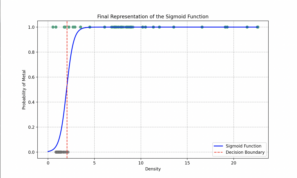
Our favorite robot has opted for the use of a linear function in his logistic regression. The optimal parameters he determined after the gradient descent are \(a = 16.85\) and \(b = 9.71\).
Analysis of the graph reveals that if the robot encounters a material with a density of 1.5, for example, it can assert with an accuracy of about 80% that it is plastic. For a density of 0.5, it can identify the material as plastic with an accuracy of 98%, while a density of 4 leads it to conclude it’s metal with an accuracy of 99%.
Thus, thanks to its logistic regression model, the robot can generally determine with an accuracy of 93% whether the provided material is metal or plastic. However, to further refine its predictions, it would be beneficial to explore more complex features in the sigmoid function, such as using polynomials with a greater number of parameters to adjust, for example.
Moreover, the model could be significantly enhanced by adopting more sophisticated algorithms than logistic regression. Approaches such as Random Forests, Support Vector Machines (SVM), or even k-Nearest Neighbors (which we will explore in the next sections) could offer optimized performance.
Another strategy to strengthen the model’s capacity would be to provide it with a broader set of features, such as electrical conductivity, thermal conductivity, etc., or to increase the amount of data. By enriching the dataset in this way, the robot could improve its understanding of existing nuances between different types of materials, leading to more accurate and robust classifications.
Beyond Waste Sorting: Determining Metal Types
Exploring deeper into the realm of metal classification, Wall-E faces a more intricate challenge: determining the specific type of metal among a variety of alloys, including bronze, gold, silver, and many others.
To tackle this challenge, Wall-E’s tool of choice becomes the k-Nearest Neighbors (KNN) algorithm.
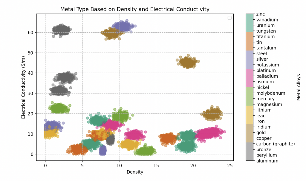
It’s worth noting that we have created the dataset from scratch by randomly selecting the features of the samples, but close enough to the fixed values of density and electrical conductivity of pure metals (which determine a metal’s ability to conduct electricity). Here is the list of all the pure metals we have recorded for Wall-E with their respective characteristics.
| Type of Metal | Electrical Conductivity (in Giga S/m) | Density |
|---|---|---|
| Steel | 1.5 | 7.500 - 8.100 |
| Aluminium | 37.7 | 2.700 |
| Silver | 63 | 10.500 |
| Beryllium | 31.3 | 1.848 |
| Bronze | 7.4 | 8.400 - 9.200 |
| Carbone (graphite) | 61 | 2.250 |
| Copper | 59.6 | 8.960 |
| Tin | 9.17 | 7.290 |
| Iron | 9.93 | 7.860 |
| Iridium | 19.7 | 22.560 |
| Lithium | 10.8 | 5.30 |
| Magnesium | 22.6 | 1.750 |
| Mercury | 1.04 | 13.545 |
| Molybdenum | 18.7 | 10.200 |
| Nickel | 14.3 | 8.900 |
| Gold | 45.2 | 19.300 |
| Osmium | 10.9 | 22.610 |
| Palladium | 9.5 | 12.000 |
| Platinium | 9.66 | 21.450 |
| Lead | 4.81 | 11.350 |
| Potassium | 13.9 | 0.850 |
| Tantalum | 7.61 | 16.600 |
| Titanium | 2.34 | 4.500 |
| Tungsten | 8.9 | 19.300 |
| Uranium | 3.8 | 19.100 |
| Vanadium | 4.89 | 6.100 |
| Zinc | 16.6 | 7.150 |
This simulates metallic alloys, where each alloy is considered to be composed of a pure metal to be determined and impurities that slightly modify its characteristics. Wall-E’s database includes 300 samples for each type of metallic alloy. Here are five of them, each characterized by its distinctive properties.
| Type of Metal | Electrical Conductivity (in Giga S/m) | Density |
|---|---|---|
| Steel | 2.7093 | 7.7446 |
| Vanadium | 5.8000 | 7.5000 |
| Iron | 9.2600 | 8.4000 |
| Gold | 43.000 | 18.500 |
| Bronze | 7.51320 | 8.7000 |
Wall-E’s goal will be to classify each metallic sample he finds based on its density and electrical conductivity into a category of pure metals.
Contrast with Binary Classification and Complexities of Multiclass Classification
Wall-E, having mastered binary classification to distinguish precious metals from plastics, realizes that the next step, multiclass classification, poses a more complex challenge. While binary classification simply divides objects into two distinct categories, such as metal or plastic, Wall-E must now differentiate between specific types. The simplicity of a decision boundary like a line, used in binary classification, is no longer sufficient.
In this new territory, Wall-E must navigate a complex feature space where metals can overlap. This complexity demands a more sophisticated approach, and this is where Wall-E turns to a method that takes into account the subtleties of relationships between metals.
The Power of Proximity: K Nearest Neighbors
In this quest, Wall-E turns to the KNN algorithm, or K Nearest Neighbors, which is a classification method based on the fundamental concept of proximity in the feature space.
The essential idea behind KNN is to group similar objects in the feature space. In our context, this means that if a piece of bronze shares similar characteristics with other pieces of bronze, these objects will be located close to each other in this multidimensional space. Wall-E skillfully exploits this notion to assign each piece of metal a label corresponding to its type.
Its operational process is quite intuitive. When a new piece of metal needs to be classified, Wall-E measures its specific characteristics, such as density, electrical conductivity, etc., thus positioning it in the feature space. The algorithm then identifies the k nearest neighbors of this new piece in this space. These neighbors are the pieces of metal that share similar characteristics.
Once the neighbors are identified, KNN assigns the new piece the type of metal that receives the most votes among these close neighbors. It’s as if each neighbor is voting for the category to which it belongs, and the type of metal with the highest number of votes is assigned to the new piece.

This flexible and proximity-based approach allows Wall-E to accurately classify metals, even without having an in-depth understanding of the specific characteristics of each type. Thus, KNN becomes an effective ally in Wall-E’s quest to determine the type of metal by harnessing the power of proximity in the feature space.
Metal Classification Process: Neighbors in Action
Wall-E searches through its relatively extensive database, which includes various types of metals and alloys, each associated with specific characteristics such as electrical conductivity, density, and other unique properties. These features constitute the dimensions of the feature space where each metal is represented. Unfortunately, Wall-E hasn’t had the time to measure all the properties of each metal and must therefore make do with only density and electrical conductivity.
When a new piece of metal comes in, Wall-E activates the KNN algorithm to determine its type. The process unfolds as follows:
• Feature Measurement: Wall-E measures the characteristics of the new piece of metal, placing it in the feature space.
• Identification of Close Neighbors: KNN identifies the k nearest neighbors of the new piece in this feature space. These neighbors are pieces of metal that share similar characteristics.
• Majority Votes: By examining the metal types of the neighbors, Wall-E assigns the new piece the type that receives the most votes among the close neighbors, i.e., the majority metal type.

This process of proximity and voting enables Wall-E to accurately classify the new piece of metal, even without an in-depth knowledge of the specific characteristics of each type. He excels at this!
Embarking on a quest in search of electronic artifacts aboard his spaceship, our intrepid explorer engages in a meticulous process of disassembly and measurement, scrutinizing the density and electrical conductivity of each unknown component. Thanks to the KNN algorithm, finely tuned with an optimal parameter k of 20 neighbors, chosen after thorough trials (see the next section), he can confidently assert his ability to identify any metal alloy with an assurance approaching 95%.
A technological feat that attests to the precision of his classifications.

The first object subjected to his analysis reveals a density of 18.5 and an electrical conductivity of 43 gigasiemens per meter. Our explorer is filled with enthusiasm, realizing that he has come across gold!
Even better, his certainty reaches an impressive score of 100%, as clearly suggested by the graph alongside.
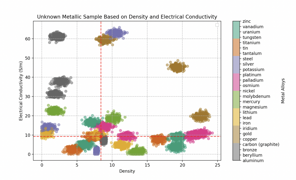
The second component capturing his attention is a grayish metal plate, displaying traces of rust. The measurements reveal a density of 8.4 and an electrical conductivity of 9.26 gigasiemens per meter.
The application of his KNN algorithm hints at a high probability of an iron alloy, with a certainty of 70%. However, a degree of uncertainty remains, leading him to also consider possibilities such as bronze (20% probable) or tin (10% probable). The mystery persists, unveiling the complexity of the discovered metallic elements.
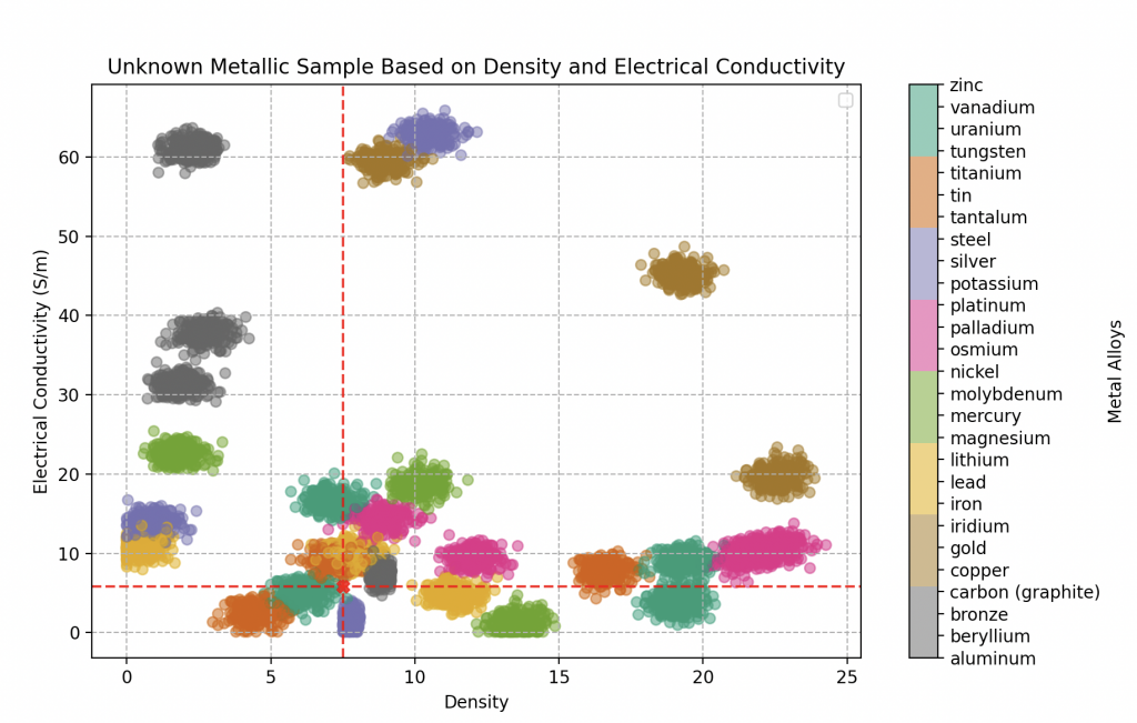
Finally, the last component, with a density of 7.5 and electrical conductivity of 5.8 gigasiemens per meter, unveils a complex metallic composition.
In-depth analysis by the KNN algorithm indicates a predominance of a particularly rare metal: vanadium, likely around 70%. It is closely followed by tin at 25%, and finally iron at a proportion of 5%.
Wall-E quickly grasps the intricacies of the analysis process, especially the complexity that arises when metals overlap on the graph. He acknowledges that predicting with absolute certainty of 100% can become challenging in these situations. However, despite these challenges, the results obtained by the KNN algorithm remain exceptional.
The algorithm’s performance in metal classification, even in scenarios where features overlap, attests to its efficiency and robustness. Thus, Wall-E can leverage this powerful technique to explore and classify various metallic components with increased confidence.
The Art of Model Selection
In the heart of its quest for sorting electronic components (Classification) and even in estimating the price of gold (Regression), the little robot becomes aware of the need to navigate with caution
Exploring New Horizons: Training and Testing
He quickly grasps the importance of never evaluating his model on the same data used for training.
To illustrate this point, let’s imagine that Wall-E is teaching young robots to analyze meteorites, offering various courses and providing practical exercises for their training, with the intention of evaluating them at the end of their school cycle.
However, Wall-E is aware that if he assesses the performance of his apprentices on the same meteorites used during his class, it would make the task too easy. The robots would simply recognize specific features they have already encountered, without a genuine understanding.

To avoid this bias, Wall-E implements a clever approach: he divides the set of exercises (his dataset) into two distinct parts, creating the training set and the test set.
The training set, typically representing 80% of the data, is dedicated to training the model; Wall-E guides the young robots through lessons and exercises using this data. On the other hand, the test set, consisting of 20% of the data, is reserved for the final evaluation of the model.
Thus, when testing the knowledge acquired by the robots on new meteorites, Wall-E ensures that they can apply their skills to novel situations, thereby avoiding mere memorization of the training data. This process ensures that the model is capable of generalizing and providing accurate predictions even on previously unseen data.
Rising to Excellence: Model Validation
Proud of his machine learning training and evaluation skills, Wall-E, as an experienced data scientist, is now dedicated to improving the accuracy of his model. To achieve this, he must adjust the model’s hyperparameters, a task similar to fine-tuning the settings of a radio antenna for optimal reception. For example, in the case of his previous model, adjusting the number of neighbors in his KNN Classifier.
However, Wall-E is aware of the pitfalls that could arise if he optimizes the model’s performance on the test set. This would render the test set data unusable for the final evaluation. To avoid this, Wall-E introduces a third section in his dataset: the validation set. This section allows him to explore model settings that offer the best performance while preserving the test set data for impartial evaluation.
When comparing different models, such as KNN Classifiers with 2, 3, 20, or even 100 neighbors, Wall-E follows a rigorous methodology. He starts by training these models on the training set. Then, he selects the model that performs the best on the validation set. Finally, to estimate real-world performance, he evaluates this chosen model on the test set.
Wall-E illustrates these choices by plotting two essential curves: performance on the training set and performance on the validation set.
The curves below represent the training and validation scores as a function of different values of the explored parameter, such as the number of neighbors in the case of KNN Classifiers.
This visualization allows for the detection of crucial trends, including model overfitting or underfitting based on the parameter values.
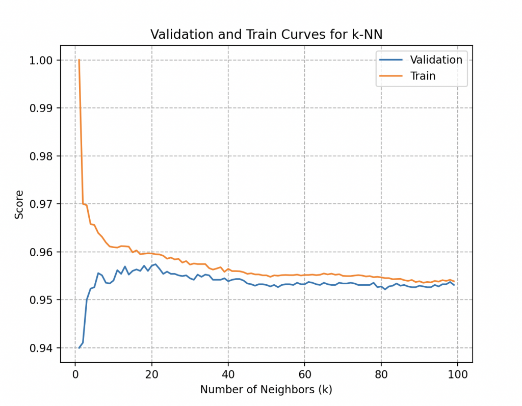
More specifically, the validation curve for the number of neighbors (k) in KNN provides answers to key questions.
• Overfitting: The significant gap between the training score and the validation score may indicate overfitting, meaning the model is too complex and loses generalization. Overfitting is an undesirable behavior in machine learning where the learning model gives accurate predictions for training data but not for new data.
• Underfitting: On the other hand, when a model has not learned the patterns in the training data well and fails to generalize correctly to new data, it is referred to as underfitting. An underfitting model performs poorly on training data and leads to unreliable predictions.
• Sensitivity to Parameter Choice: Observing variations in model performance with different values of the number of neighbors allows Wall-E to choose an optimal value for k, maximizing model performance.
By adopting this systematic approach, Wall-E ensures making informed decisions for the optimal configuration of his model, avoiding the pitfalls of overfitting or underfitting and ensuring optimal performance in real-world contexts.
In his case, both curves quickly reach an accuracy score of 95.7% from around 20 to 25 neighbors and plateau around this value as the number of neighbors increases. A detailed analysis of the curves (which we won’t go into here) would indicate that the optimal score is achieved with 20 neighbors.
Although he has a deep understanding of the process, Wall-E knows there’s one crucial detail remaining: how to ensure the dataset split is the best? He finds the solution in cross-validation.
The Dance of Models: Cross-Validation
Wall-E employs a clever cross-validation methodology to enhance the robustness of his model selection. Specifically, he embraces the K-fold method, where the dataset is split into K parts (here, 5 parts). During training, Wall-E’s model is systematically trained on K-1 of these partitions and validated on the remaining partition, repeating this process K times. This ensures a more reliable and stable evaluation of the model’s performance, making sure that no particular partition overly influences the results.
Furthermore, Wall-E also leverages Stratified K-fold, an intelligent variant of K-fold that takes into account the class distribution in the dataset. This approach ensures that each fold maintains a proportional representation of all classes, crucial when classes are not evenly distributed. Thus, Wall-E ensures a robust model selection, resistant to variations in data splitting, while also considering class distribution for even more precise evaluation.
There are, of course, other data splitting strategies that may adapt more or less effectively depending on the available data, which we will discuss in a future article.
The Learning Waves: Learning Curves
Eager to determine if his model could benefit from improvement through the addition of more data, Wall-E delves into a more thorough exploration by examining learning curves.
These curves provide a visual representation of how the model’s performance evolves based on the amount of training data provided. While adding data may initially lead to performance improvement, Wall-E has the insight to recognize that these benefits eventually reach a threshold. Understanding when the model reaches its limits becomes invaluable wisdom, allowing for a judicious use of time and resources.

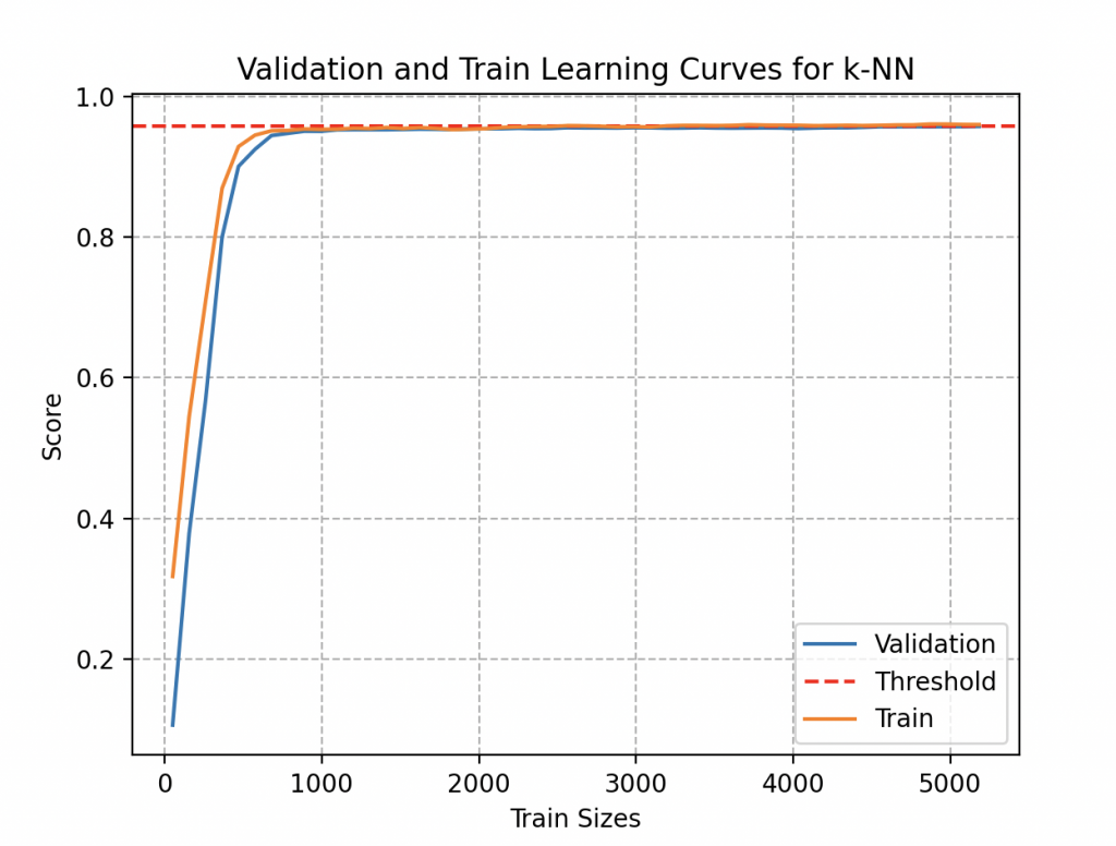
Examining this curve, he notices that a sufficiently accurate estimation could have been obtained using fewer than 1000 metal samples, roughly around 37 alloys of each type. Even by accumulating 300 metal samples for each type (300 times 27, totaling 8100 objects), he observes that it brings little significant improvement to his model (its accuracy plateaus at 95.7%). Fortunately, he collects data for the joy of it!
Thus, Wall-E gracefully dances to the rhythm of the learning waves, navigating with finesse through the complex landscape of model selection. By mastering the intricacies of learning curves, Wall-E ensures he makes the most of his model improvement process.
The End of a Trilogy, the Beginning of a Technological Era
This final episode marks the moving conclusion of the captivating saga of the little robot Wall-E, an adventure that began with the fundamentals of machine learning and supervised learning. From his first steps into the realm of artificial intelligence, Wall-E has evolved through various chapters, exploring the basics of machine learning, delving into the in-depth study of regression, and finally, climbing the complex peaks of classification.
The first step saw Wall-E learn the ins and outs of supervised learning, a discipline that allowed him to understand how to use a database to train a model. This inaugural phase laid the groundwork for his quest to understand the complex world of data and algorithms.
The second act of this saga immersed the robot in the universe of regression, where he learned to predict continuous values based on input variables (gold based on its purity). This chapter expanded his horizons, leading him to master concepts such as gradient descent and cost function, essential tools in his machine learning toolkit.
Finally, the last episode saw our budding data scientist confront classification, an even more complex challenge involving the distinction between different types of electronic components. Modest beginnings with binary sorting (metal-plastic) evolved into a bold exploration of multi-class classification (sorting precious metals), highlighting techniques such as the K Nearest Neighbors algorithm and meticulous model selection.
Thus, this poignant conclusion of Wall-E’s saga symbolizes not only the end of an exceptional story but also the realization of gradual and methodical learning in the vast realm of machine learning. The little waste-sorting robot has traversed an impressive path, from understanding basic concepts to mastering sophisticated techniques, leaving behind a legacy of learning and perseverance. This saga, rich in lessons, concludes with the certainty that Wall-E is now ready to face new challenges in the complex world of artificial intelligence. Who knows, perhaps one day he will match EVE, paving the way for new explorations and discoveries.

Bibliography
G. James, D. Witten, T. Hastie et R. Tibshirani, An Introduction to Statistical Learning, Springer Verlag, coll. « Springer Texts in Statistics », 2013.
D. MacKay, Information Theory, Inference, and Learning Algorithms, Cambridge University Press, 2003.
T. Mitchell, Machine Learning, 1997.
F. Galton, Kinship and Correlation, Statistical Science, Institute of Mathematical Statistics, vol. 4, no 2, 1989, p. 80–86, 1989.
C. Bishop, Pattern Recognition And Machine Learning, Springer, 2006.
G. Saint-Cirgue, Machine Learnia, Youtube Channel.
J. Tolles, W-J. Meurer, Logistic Regression Relating Patient Characteristics to Outcomes. JAMA. 316 (5): 533–4, 2016.
B-V. Dasarathy, Nearest Neighbor (NN) Norms: NN Pattern Classification Techniques, 1991.
G. Shakhnarovich, T. Darrell, P. Indyk, Nearest-Neighbor Methods in Learning and Vision, 2005.
Hastie, Tibshirani, Friedman, The elements of statistical learning. Springer. p. 195, 2009.
S. Konishi, G. Kitagawa, Information Criteria and Statistical Modeling, Springer, 2008.
import pandas as pd
import numpy as np
import matplotlib.pyplot as plt
import os
print("Current Working Directory:", os.getcwd())

from sklearn.pipeline import make_pipeline
from sklearn.preprocessing import StandardScaler
from sklearn.linear_model import LogisticRegression
from sklearn.model_selection import train_test_split, GridSearchCV
from sklearn.preprocessing import OrdinalEncoder


# Replace 'path/to/your/excel/file.xlsx' with the actual path to your Excel file
excel_file_path = 'PlasticMetal_data.xlsx'

# Read the Excel file
result_df = pd.read_excel(excel_file_path)

# Display the Pandas DataFrame
print(result_df)


X = result_df['Density']
y = result_df['Material']

# Data preparation
X_train, X_test, y_train, y_test = train_test_split(X, y, test_size=0.2, random_state=42)

# Convert labels to the appropriate format for binary classification
ordinal_encoder = OrdinalEncoder(categories=[['Plastic', 'Metal']])
y_train_encoded = ordinal_encoder.fit_transform(y_train.values.reshape(-1, 1))
y_test_encoded = ordinal_encoder.transform(y_test.values.reshape(-1, 1))

# Reshape y_train and y_test
y_train_reshaped = y_train_encoded.ravel()
y_test_reshaped = y_test_encoded.ravel()

# Reshape X_train and X_test
X_train_reshaped = X_train.values.reshape(-1, 1)
X_test_reshaped = X_test.values.reshape(-1, 1)

# Create the model
model = make_pipeline(StandardScaler(), LogisticRegression(random_state=42))

print(model)

# Create parameter dictionary
params = {
    'logisticregression__penalty': ['l2', None],
    'logisticregression__solver': ['lbfgs'],
    'logisticregression__max_iter': [100, 200, 300, 500, 1000]
}

# Create a search grid
grid = GridSearchCV(model, param_grid=params, cv=5)

# Train the model
grid.fit(X_train_reshaped, y_train_reshaped)

print(grid.best_params_)
print(grid.best_score_)

modelB = grid.best_estimator_

# Model evaluation
accuracy = modelB.score(X_test_reshaped, y_test_reshaped)
print(f"Model accuracy: {accuracy}")

# Predictions
predictions = modelB.predict(X_test_reshaped)

print(predictions)
print(ordinal_encoder.inverse_transform(np.array([[1], [0]])))

coefficients = modelB.named_steps['logisticregression'].coef_
intercept = modelB.named_steps['logisticregression'].intercept_

print("Coefficients:", coefficients)
print("Intercept:", intercept)

# Plot the sigmoid function with normalized data
density_values = np.linspace(0, X_train_reshaped.max(), 300).reshape(-1, 1)
probabilities = modelB.predict_proba(density_values)[:, 1]

# Find the density corresponding to a probability of 0.5
decision_boundary = density_values[np.argmax(probabilities >= 0.5)]

# Plot the sigmoid function
plt.figure(figsize=(10, 6))
plt.scatter(X_train_reshaped, y_train_reshaped, c=y_train_reshaped, cmap='Dark2_r', alpha=0.5)
plt.plot(density_values, probabilities, color='blue', linewidth=2, label='Sigmoid Function')
# Add the vertical line corresponding to a probability of 0.5
plt.axvline(x=decision_boundary, color='red', linestyle='--', label='Decision Boundary')
plt.title('Final Representation of the Sigmoid Function')
plt.xlabel('Density')
plt.ylabel('Probability of Metal')
plt.grid(ls='--')
plt.legend()
plt.show()

# Suppose you have a new material with a certain density
new_material_density = 4  # Replace this value with the actual density of your new material

new_material_density_reshaped = np.array(new_material_density).reshape(-1, 1)

print(modelB.predict(new_material_density_reshaped))

# Make the prediction with the model
probability_of_metal = modelB.predict_proba(new_material_density_reshaped)[:, 1]

# Display the result
print("Probability of being metal:", probability_of_metal)
import pandas as pd
import numpy as np
import matplotlib.pyplot as plt
import os
print("Current Working Directory:", os.getcwd())


from sklearn.pipeline import make_pipeline
from sklearn.preprocessing import MinMaxScaler
from sklearn.neighbors import KNeighborsClassifier
from sklearn.model_selection import train_test_split, GridSearchCV, validation_curve, learning_curve
from sklearn.preprocessing import LabelEncoder


# Replace 'path/to/your/excel/file.xlsx' with the actual path to your Excel file
excel_file_path = 'metals_samples.xlsx'

# Read the Excel file
result_metals_df = pd.read_excel(excel_file_path)

# Display the Pandas DataFrame
print(result_metals_df)


X = result_metals_df[['Density', 'Electrical Conductivity']]
y = result_metals_df['Metal Type']


# Data preparation
X_train, X_test, y_train, y_test = train_test_split(X, y, test_size=0.2, random_state=42)

# Convert labels to the appropriate format for binary classification
label_encoder = LabelEncoder()
y_train_encoded = label_encoder.fit_transform(y_train)
y_test_encoded = label_encoder.transform(y_test)

# Create the model
model = make_pipeline(MinMaxScaler(), KNeighborsClassifier())

print(model)

# Create parameter dictionary
params = {
    'kneighborsclassifier__n_neighbors': [2,3,4,5,6,7,8,9,10, 15, 20, 25, 30, 40,  100],
    'kneighborsclassifier__weights': ['uniform', 'distance'],
    'kneighborsclassifier__p': [1, 2]
}

# Create a search grid
grid = GridSearchCV(model, param_grid=params, cv=5)

# Train the model
grid.fit(X_train, y_train_encoded)

print(grid.best_params_)
print(grid.best_score_)

modelB = grid.best_estimator_

# Model evaluation
accuracy = modelB.score(X_test, y_test_encoded)
print(f"Model Accuracy: {accuracy}")

# Predictions
predictions = modelB.predict(X_test)


#for i in range(0, 32):
    #print(label_encoder.inverse_transform(np.array([i])))


# Sample
X_sample = pd.DataFrame({'Density': [7.5], 'Electrical Conductivity': [5.8], 'Metal Type' : [np.NaN]})
X_sample = X_sample[['Density','Electrical Conductivity']]


# Predict using the scaled sample
prediction = modelB.predict(X_sample)
prediction_proba = modelB.predict_proba(X_sample)

print("Predicted Metal Type:", label_encoder.inverse_transform(prediction))
print("Prediction Probabilities:", prediction_proba)

# Probability Prediction
prediction_proba = modelB.predict_proba(X_sample)


# Validation Curves

k_range = np.arange(1,100)

#train_score, val_score = validation_curve(model, X_train, y_train_encoded, param_name='kneighborsclassifier__n_neighbors',param_range=k_range, cv =5)

#plt.plot(k_range,val_score.mean(axis=1), label='Validation')
#plt.plot(k_range,train_score.mean(axis=1), label='Train')
#plt.xlabel('Number of Neighbors (k)')
#plt.ylabel('Score')
#plt.grid(ls='--')
#plt.legend()
#plt.title('Validation and Train Curves for k-NN')
#plt.show()

# Learning curves

#N, learn_train_score, learn_val_score = learning_curve(modelB, X_train, y_train_encoded, train_sizes=np.linspace(0.01, 1.0, 50), cv = 5)

#print(N)
#plt.plot(N,learn_val_score.mean(axis=1), label='Validation')
#plt.axhline(y=0.957, c='red', ls='--', label = 'Threshold')
#plt.plot(N,learn_train_score.mean(axis=1), label='Train')
#plt.xlabel('Train Sizes')
#plt.ylabel('Score')
#plt.grid(ls='--')
#plt.legend()
#plt.title('Validation and Train Learning Curves for k-NN')
#plt.show()


# Displaying probabilities with class names
for i, metal_class in enumerate(label_encoder.classes_):
    print(f"Probability for class '{metal_class}': {prediction_proba[0, i]}")


plt.figure(figsize=(10, 6))
scatter = plt.scatter(X_train['Density'], X_train['Electrical Conductivity'], c=y_train_encoded, cmap='Dark2_r', alpha=0.5)
plt.scatter(X_sample['Density'], X_sample['Electrical Conductivity'], c='red', s=50, marker='X', alpha=0.8)
plt.axvline(x=tuple(X_sample['Density']), c='red', ls='--', alpha=0.8)
plt.axhline(y=tuple(X_sample['Electrical Conductivity']), c='red', ls='--', alpha=0.8)
plt.xlabel('Density')
plt.ylabel('Electrical Conductivity (S/m)')
plt.grid(ls='--')
# Configure the colorbar correctly
cbar = plt.colorbar(scatter, ticks=range(len(label_encoder.classes_)))
cbar.set_label('Metal Alloys')
cbar.set_ticklabels(label_encoder.classes_)
plt.title('Unknown Metallic Sample Based on Density and Electrical Conductivity')
plt.legend()
plt.show()