Waste Allocation Load Lifter: Earth Class

As a robot faithful to its mission and amidst occasional gold estimations, Wall-E does not forget its primary task: sorting waste. It is during its expeditions to remote corners of the planet that he encounters the ultimate challenge that stimulates his curious mind. Among the objects he gathers, Wall-E comes across a diverse collection of old electronic components — some in good condition that he brings back to the base, and others defective that he stores in a corner.

Passionate about such objects, he begins to unscrew, pull apart, and carefully categorize each component into two distinct categories (binary classification): on one side the precious metal pieces (multiclass classification), and on the other the worthless plastic. The fundamental question is: how does he accomplish such a mission?

It is strongly recommended to have read Episodes I and II before continuing!

Wall-E’s New Horizons: Classification

The epic journey of our intrepid lone robot, Wall-E, takes on a fascinating new dimension as he explores the vast realm of classification. After brilliantly mastering the art of regression in the previous episode (see Wall-E: The Little Gold Miner), Wall-E courageously embarks on a new phase by delving into binary classification between precious metals and plastics. This first preparatory step marks the beginning of a more complex quest, where Wall-E boldly deploys his classification skills.

Building on his initial successes, Wall-E decides to broaden his scope by tackling the multi-class classification of metals, making the K-Nearest Neighbors (KNN) algorithm his preferred ally. This new challenge requires Wall-E to gain a deeper understanding, as he must not only distinguish between two categories but also classify different types of metals such as bronze, gold, and silver.

The Key Element: Always the Data

Meeting the Samples

Each example $k$ was an element with specific characteristics, such as density $x^{(k)}$, thermal conductivity $x_2^{(k)}$, electrical conductivity $x_3^{(k)}$, etc. To illustrate our case simply, we will consider only the density variable $x^{(k)}$.

For each sample $k$, Wall-E notes whether it is a metal (labeled $y^{(k)}=1$) or plastic (labeled $y^{(k)}=0$). Here is a concrete example of 5 samples (among the 650 he already knows):

Sample	Density	Material
1	2.165747	Plastic
2	7.151579	Metal
3	0.901240	Plastic
4	19.24357	Metal
5	12.54564	Metal

Decision Boundaries

The difference with the previous problem is that here we need to define what we call a decision boundary. Instead of looking at each object individually, Wall-E decides to divide this space into different regions. Each region is intended to receive a specific type of object, either metal or plastic. The limits of these regions define decision boundaries.

When Wall-E draws these boundaries, he wants to ensure that similar objects fall in the same region. Ideally, the two groups should be perfectly separated, as if in distinct boxes. A simple straight line could do the trick.

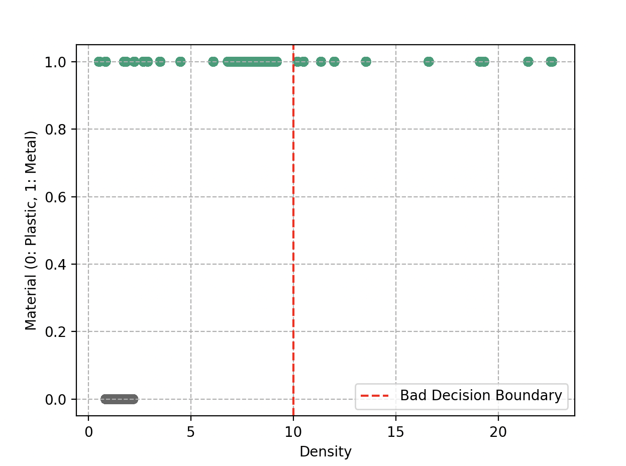
However, reality is not always so simple. Sometimes objects end up on the wrong side of the line. Wall-E is also aware that he should not draw zigzagging, overly complex boundaries — that would lead to overfitting.

Building the Binary Classification Model

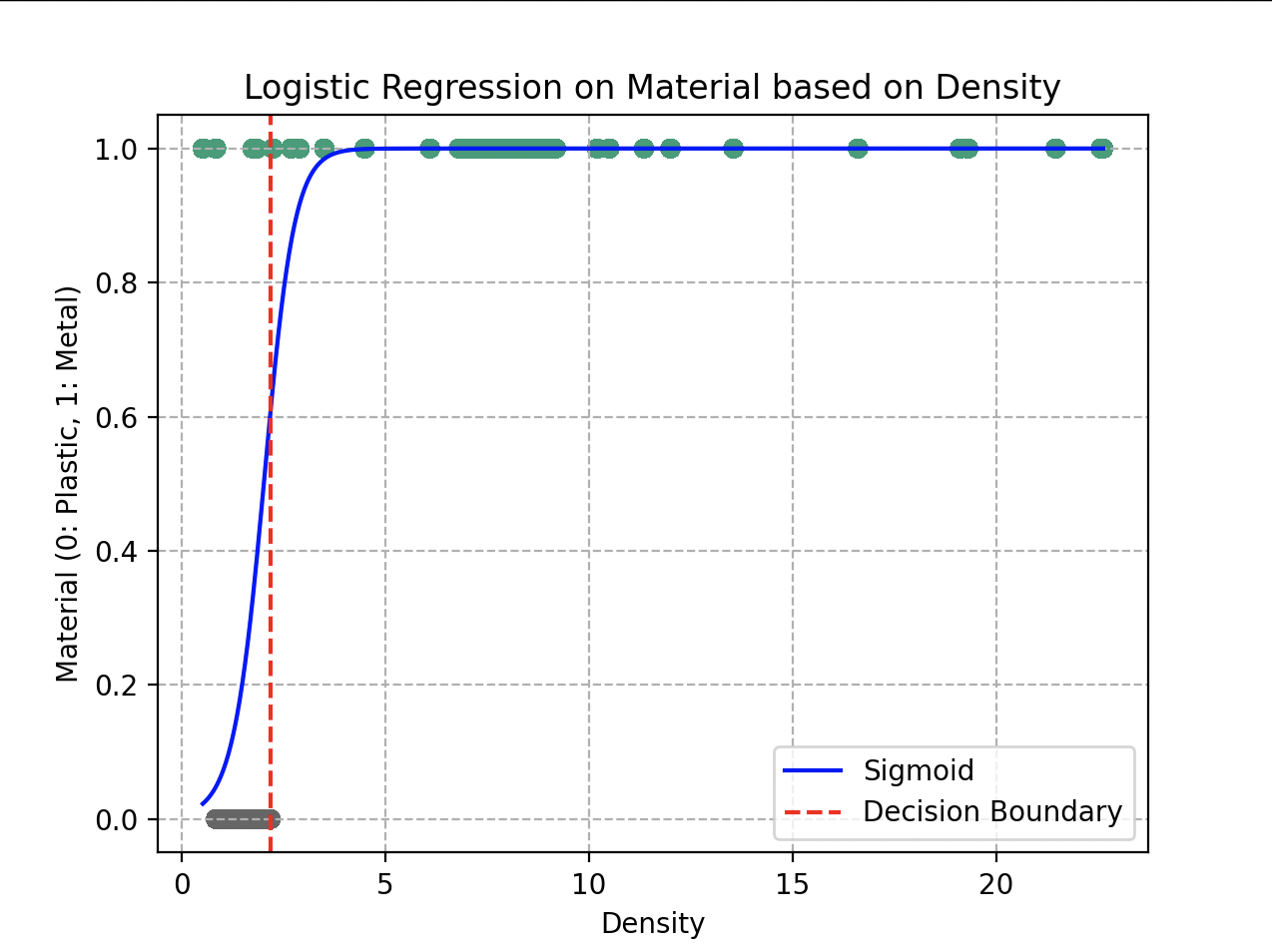
Wall-E chooses a classic logistic regression model whose associated function (ranging between 0 and 1) is expressed as:

$$\sigma(x) = \frac{1}{1+\exp(-x)}$$

This is the sigmoid function (named for its “S” shape).

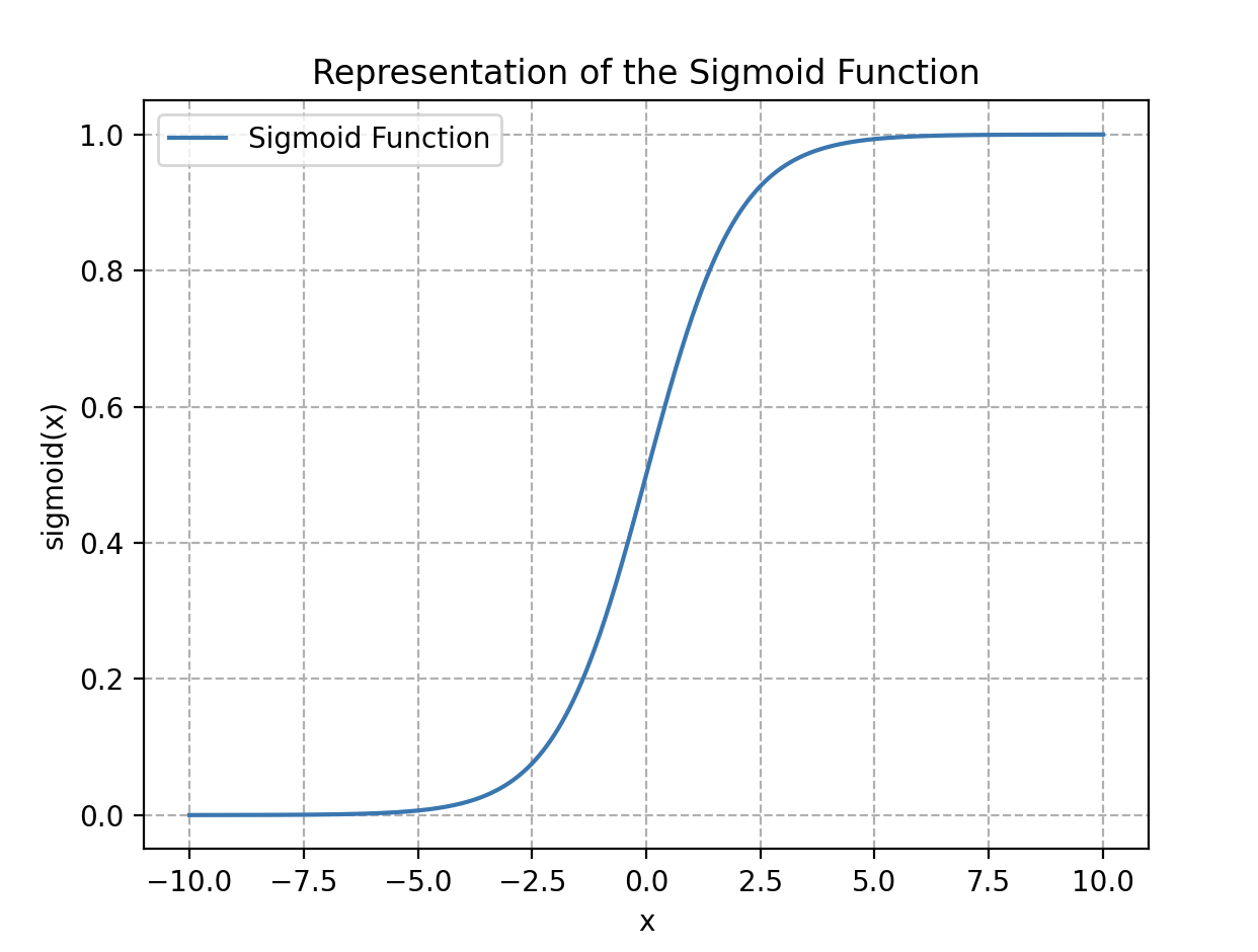
The logistic / sigmoid function.

Applied to our dataset, we obtain $\sigma(z) = \frac{1}{1+\exp(-z)}$, where $z$ can be a linear function $ax+b$ or a polynomial $ax^2 + bx + c$, with $a$, $b$, and $c$ as parameters to fit.

The big advantage of such a function is that we can easily define a decision boundary by setting a decision threshold value. If the probability is greater than 0.5, we classify the object as “metal”; below 0.5, as plastic.

Evaluating Predictions: the Cost Function

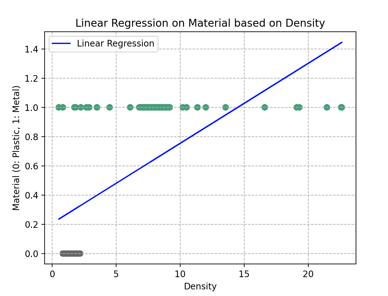
Wall-E builds his model, but he wants to evaluate the accuracy of his predictions. He could use a classic regression cost function, MSE (see Wall-E: The Little Gold Miner):

$$\text{MSE}(a, b) = \frac{1}{n}\sum_{k=1}^{n}\left(\sigma(x^{(k)}) - y^{(k)}\right)^2.$$

However, this cost function is not convex; it has multiple local minima. This makes gradient descent inefficient — using the mountain-relief analogy, Wall-E might get trapped in a local minimum that is not necessarily the global one.

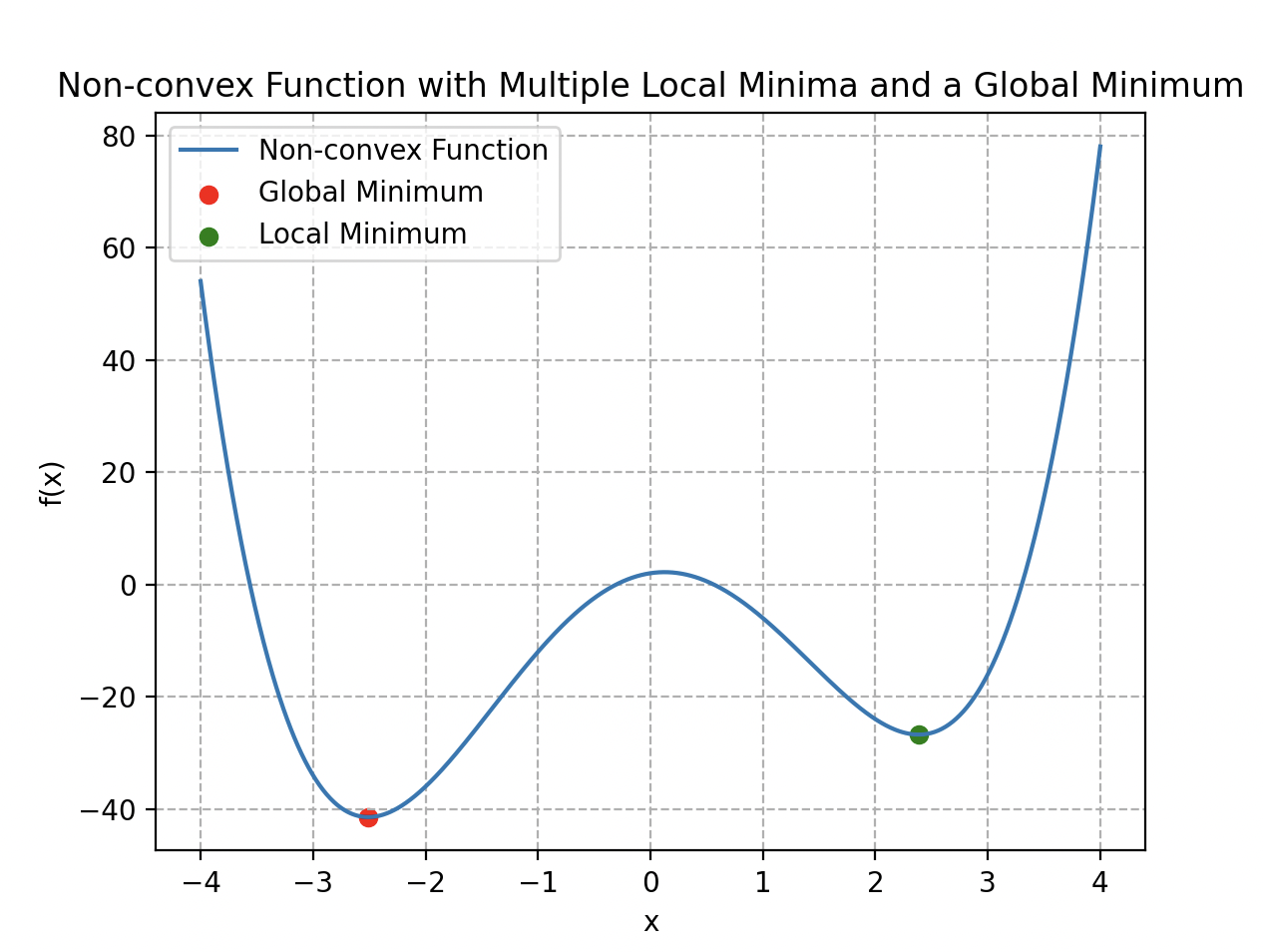
A non-convex function with several local minima and one global minimum.

Wall-E therefore introduces a new cost function based on the logarithm (negative log-likelihood):

$$L(a,b) = -\frac{1}{n}\sum_{k=1}^n\left[y^{(k)}\log\left\{\sigma\left(ax^{(k)}+b\right)\right\} + \left(1-y^{(k)}\right)\log\left\{1-\sigma\left(ax^{(k)}+b\right)\right\}\right]$$

This function has the convexity property, meaning it has a single global minimum and no local minima. This makes gradient descent much more reliable for adjusting model parameters.

The first part of the cost function, when a label is 1, is represented by $-y^{(k)}\log\left\{\sigma\left(x^{(k)}\right)\right\}$. The second part handles the case where the label is 0: $-\left(1-y^{(k)}\right)\log\left\{1-\sigma\left(x^{(k)}\right)\right\}$.

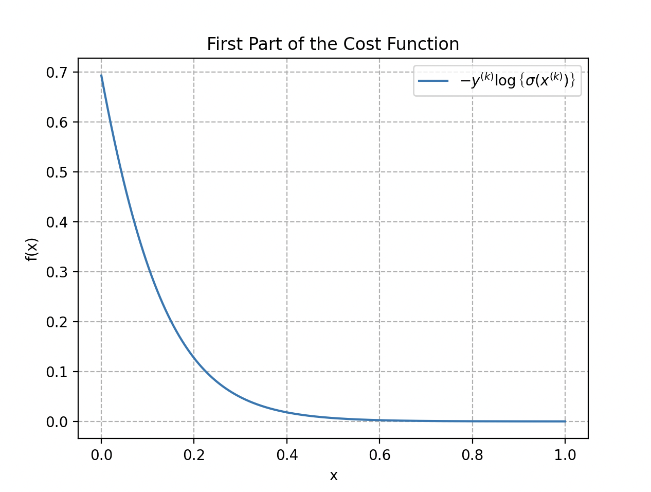
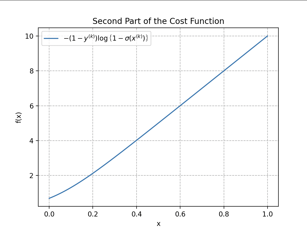
When $y^{(k)}=1$, only the first part of the function acts; when $y^{(k)}=0$, only the second one. The total cost function is the average of these two parts, taken over all $n$ training examples, to obtain a global measure of how well the model fits the training data.

Re-Descending the Gradient

We do exactly the same thing as for regression but with the new cost function. The gradients are:

$$\frac{\partial L(a, b)}{\partial a} = \frac{1}{n}\sum_{k=1}^n\left(\sigma\left(ax^{(k)}+b\right) - y^{(k)}\right)x^{(k)}$$ $$\frac{\partial L(a, b)}{\partial b} = \frac{1}{n}\sum_{k=1}^n\left(\sigma\left(ax^{(k)}+b\right) - y^{(k)}\right)$$

Parameter updates:

$$a^* = a - \delta \times \frac{\partial L(a, b)}{\partial a}, \quad b^* = b - \delta \times \frac{\partial L(a, b)}{\partial b}$$

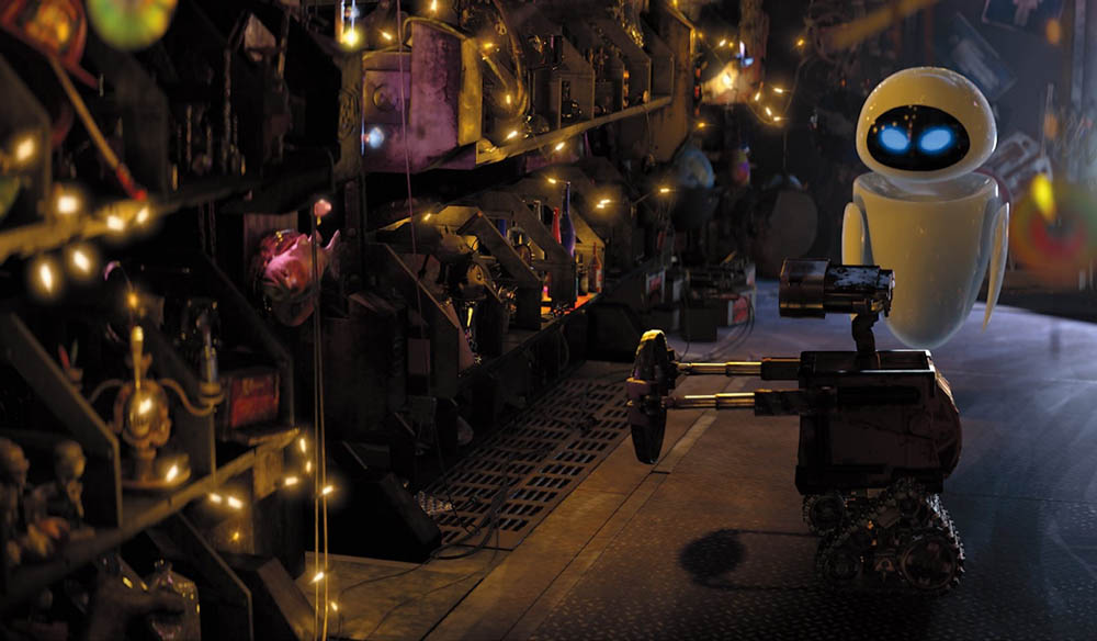
Credits: Disney/PIXAR

The Power of the Little Waste Sorter

In matrix notation, with the vector $\mathbf{Y}$, the matrix $\mathbf{X}$, and the parameter vector $\mathbf{P} = \begin{bmatrix} a \\ b \end{bmatrix}$, the sigmoid is applied component-wise:

$$\mathbf{\sigma(X \times P)} = \begin{bmatrix} \frac{1}{1+\exp(-(ax^{(1)}+b))} \\ \frac{1}{1+\exp(-(ax^{(2)}+b))} \\ \vdots \\ \frac{1}{1+\exp(-(ax^{(n)}+b))} \end{bmatrix}.$$

The cost function becomes:

$$L(\mathbf{P}) = -\frac{1}{n}\left[\mathbf{Y} \cdot \log\left\{\sigma(\mathbf{X} \times \mathbf{P})\right\} + (\mathbf{1}-\mathbf{Y}) \cdot \log\left\{1-\sigma(\mathbf{X} \times \mathbf{P})\right\}\right]$$

and its gradient:

$$\frac{\partial}{\partial \mathbf{P}} L(\mathbf{P}) = \frac{1}{n}\mathbf{X} \cdot \left(\sigma(\mathbf{X} \times \mathbf{P}) - \mathbf{Y}\right)$$

with the update rule:

$$\mathbf{P^*} = \mathbf{P} - \delta \frac{\partial}{\partial \mathbf{P}} L(\mathbf{P})$$

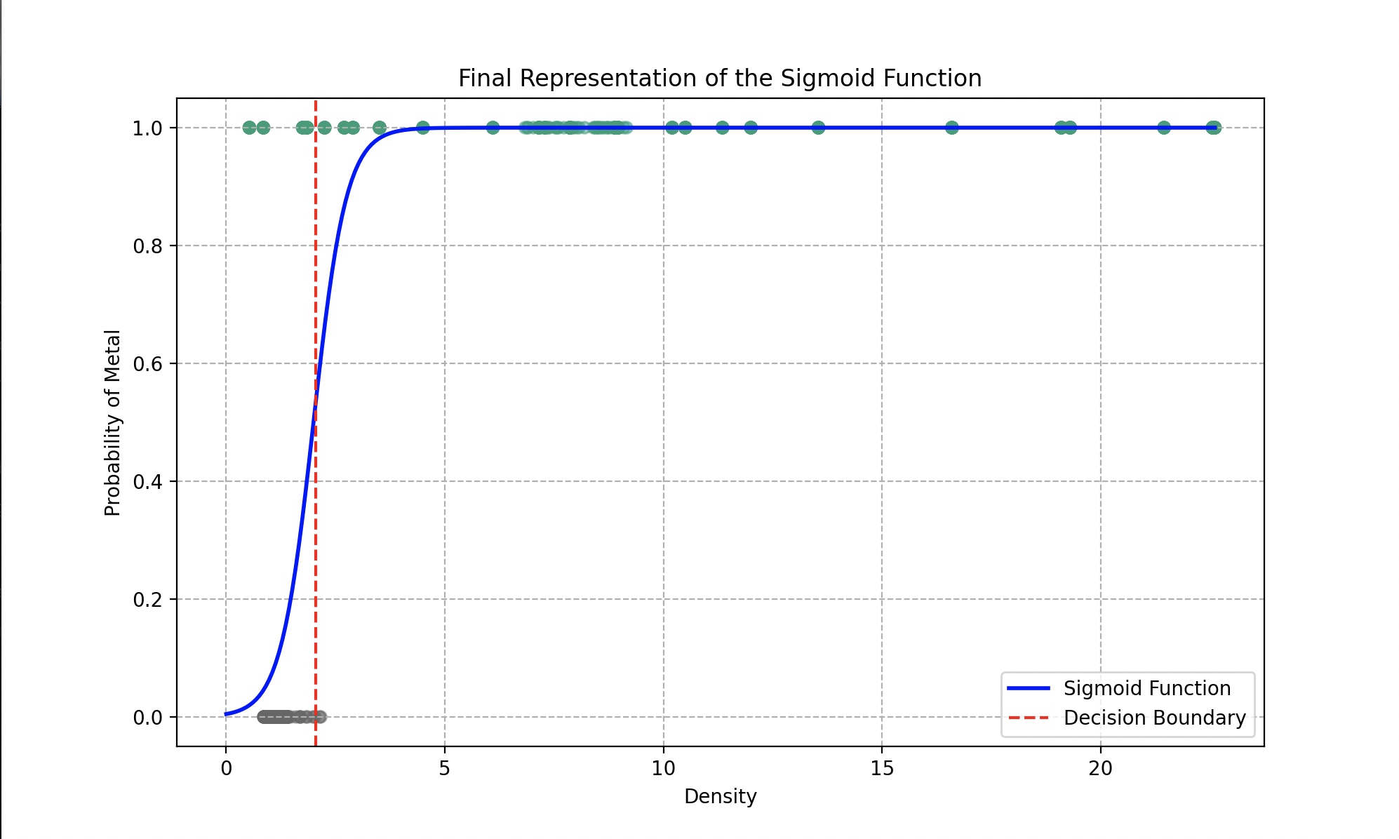
Final fit of the sigmoid function on the data.

The optimal parameters obtained after gradient descent are $a = 16.85$ and $b = 9.71$. The model can determine, with an overall accuracy of 93%, whether the supplied material is metal or plastic.

Beyond Waste Sorting: Determining the Type of Metal

Diving deeper into metal classification, Wall-E confronts a more complex challenge: determining the specific type of metal among a wide variety of alloys including bronze, gold, silver, and many others.

To meet this challenge, Wall-E’s tool of choice becomes the K-Nearest Neighbors (KNN) algorithm. Here is the list of all pure metals in Wall-E’s reference table:

Metal	Electrical Conductivity (Giga S/m)	Density
Steel	1.5	7.500 - 8.100
Aluminum	37.7	2.700
Silver	63	10.500
Beryllium	31.3	1.848
Bronze	7.4	8.400 - 9.200
Carbon (graphite)	61	2.250
Copper	59.6	8.960
Tin	9.17	7.290
Iron	9.93	7.860
Iridium	19.7	22.560
Lithium	10.8	5.30
Magnesium	22.6	1.750
Mercury	1.04	13.545
Molybdenum	18.7	10.200
Nickel	14.3	8.900
Gold	45.2	19.300
Osmium	10.9	22.610
Palladium	9.5	12.000
Platinum	9.66	21.450
Lead	4.81	11.350
Potassium	13.9	0.850
Tantalum	7.61	16.600
Titanium	2.34	4.500
Tungsten	8.9	19.300
Uranium	3.8	19.100
Vanadium	4.89	6.100
Zinc	16.6	7.150

This simulates metallic alloys, where each alloy is composed of a pure metal to be determined plus impurities slightly modifying its characteristics. Wall-E’s database has 300 samples for each type of metallic alloy. Here are five samples, each with its distinctive properties:

Metal	Electrical Conductivity (Giga S/m)	Density
Steel	2.7093	7.7446
Vanadium	5.8000	7.5000
Iron	9.2600	8.4000
Gold	43.000	18.500
Bronze	7.5132	8.7000

Wall-E’s goal is therefore to classify each metallic sample he finds — based on its density and electrical conductivity — into one of the pure-metal categories.

Contrast with Binary Classification: the Complexity of Multi-Class

After mastering binary classification to distinguish precious metals from plastics, Wall-E realizes that the next step — multi-class classification — is a more complex challenge. Where binary classification simply splits objects into two distinct categories, Wall-E must now differentiate between many specific types. The simple decision boundary of a straight line is no longer enough.

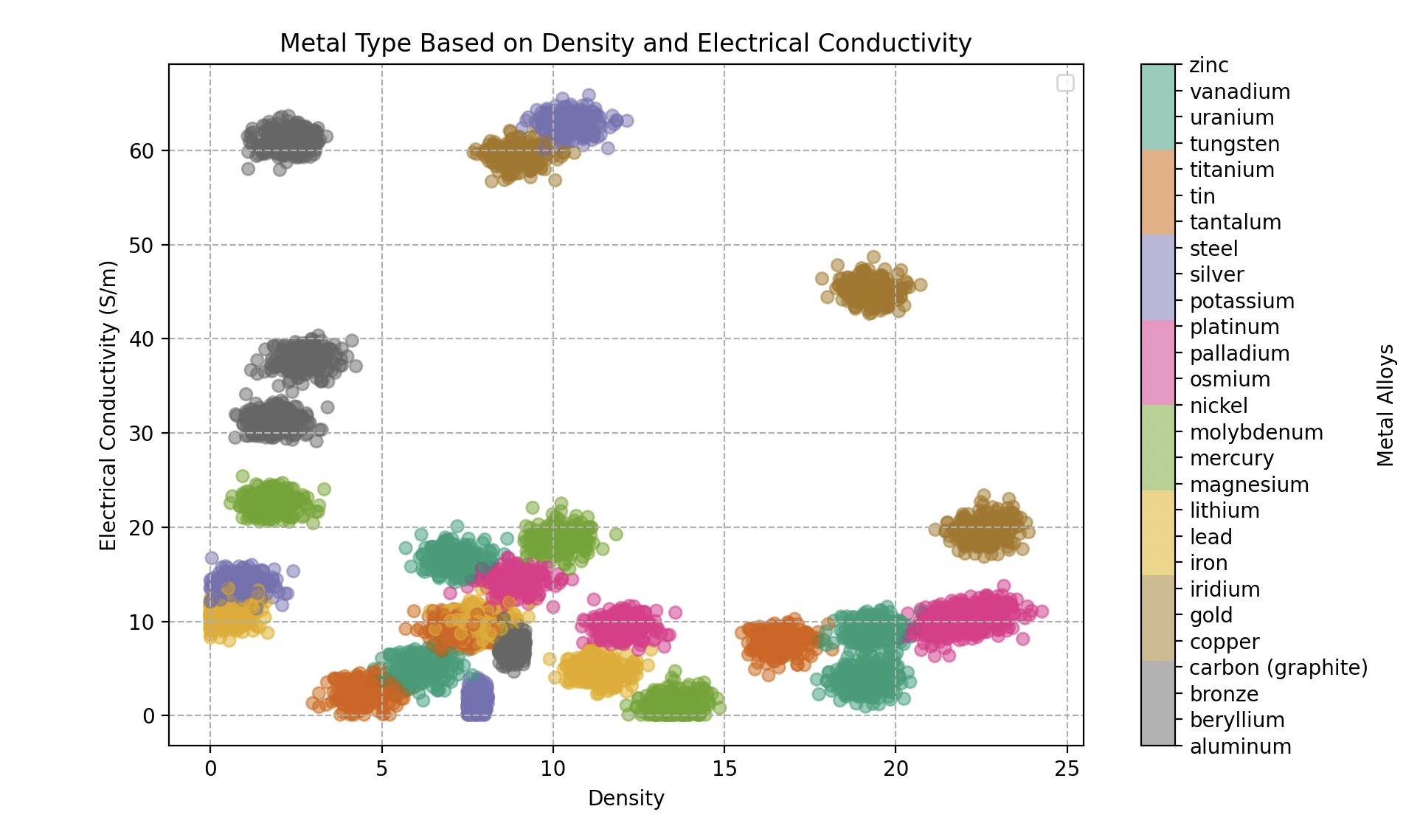
Type of metal as a function of density and electrical conductivity (Giga Siemens per meter). 300 samples for each alloy.

In this new territory, Wall-E must navigate a complex feature space where metals can overlap. This complexity requires a more refined approach — and this is where Wall-E turns to a method that takes the subtleties of relationships between metals into account.

The Power of Proximity: K-Nearest Neighbors

The essential idea behind KNN is to group similar objects in feature space. In our context, if a piece of bronze shares similar characteristics with other bronze pieces, those objects will be located near each other in this multidimensional space.

The process is fairly intuitive. When a new piece of metal must be classified, Wall-E measures its specific characteristics and positions it in feature space. The algorithm then identifies the $k$ nearest neighbors, and KNN assigns to the new piece the type of metal that gathers the most votes among those neighbors.

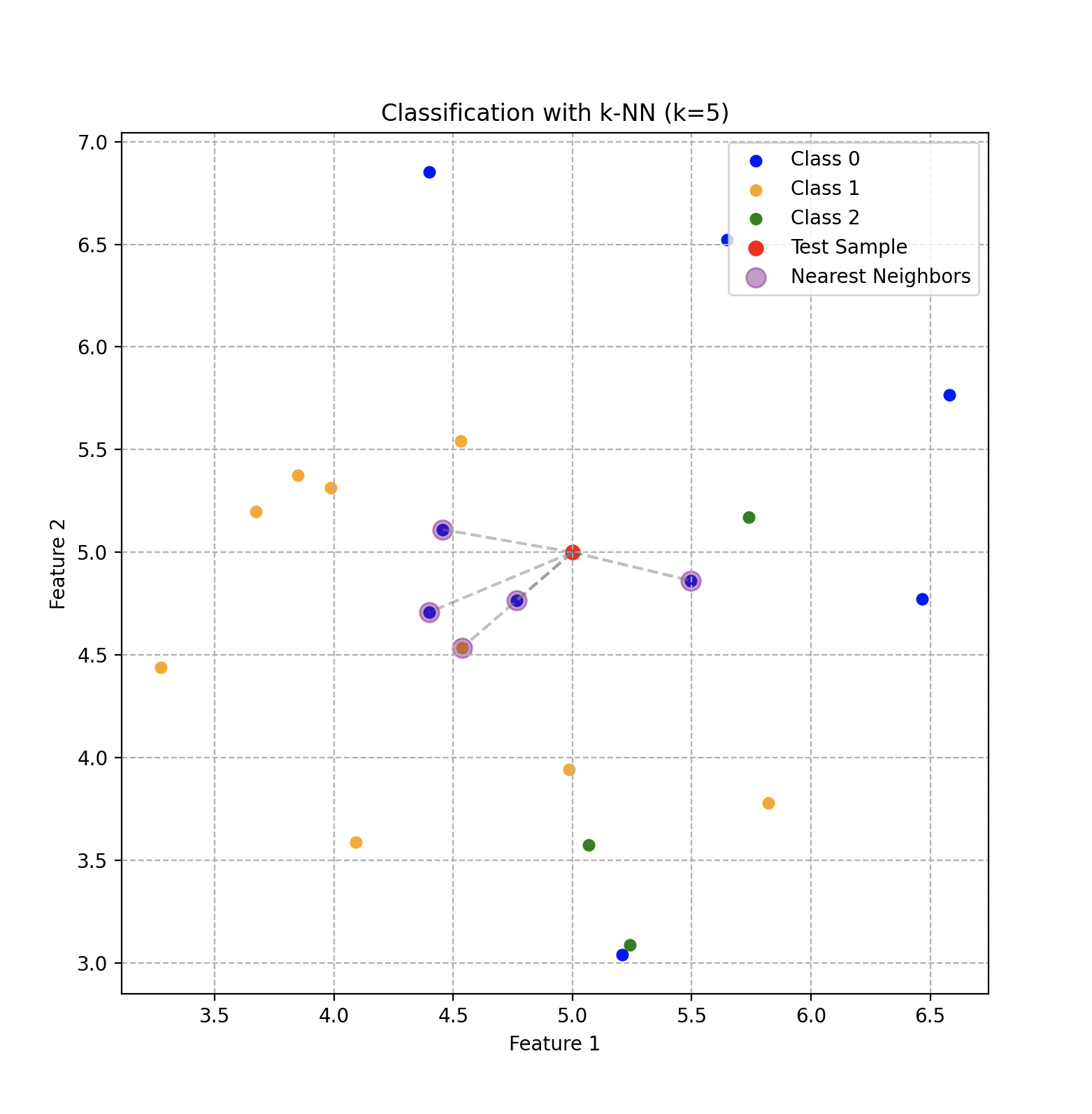
Classification using the KNN algorithm with 5 neighbors and 3 classes that depend on two features.

Metal Classification in Action: the Neighbors at Work

Wall-E searches his fairly extensive database, comprising various types of metals and alloys, each associated with specific characteristics such as electrical conductivity, density, and other unique properties. When a new piece of metal arrives, Wall-E activates the KNN algorithm:

• Feature measurement: Wall-E measures the characteristics of the new piece, placing it in feature space.
• Nearest-neighbor identification: KNN identifies the $k$ nearest neighbors of the new piece in this space.
• Majority vote: Wall-E assigns to the new piece the most common metal type among its nearest neighbors.

Credits: Disney/PIXAR

With an optimal parameter $k = 20$ neighbors, Wall-E can claim with around 95% confidence to identify any metallic alloy.

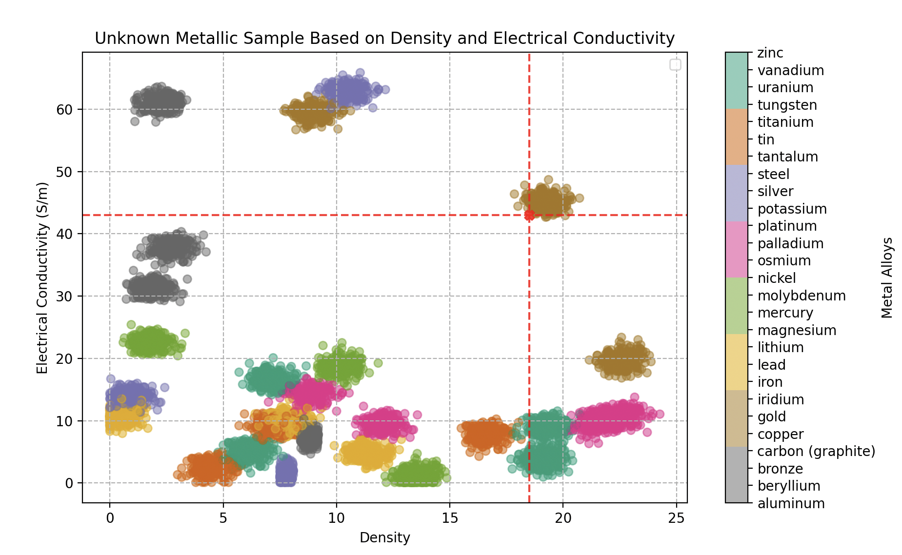
Classifying an unknown metallic sample by its density and electrical conductivity — turns out to be a gold alloy.

• The first object analyzed (density 18.5, conductivity 43 GS/m) is identified as gold with 100% confidence.

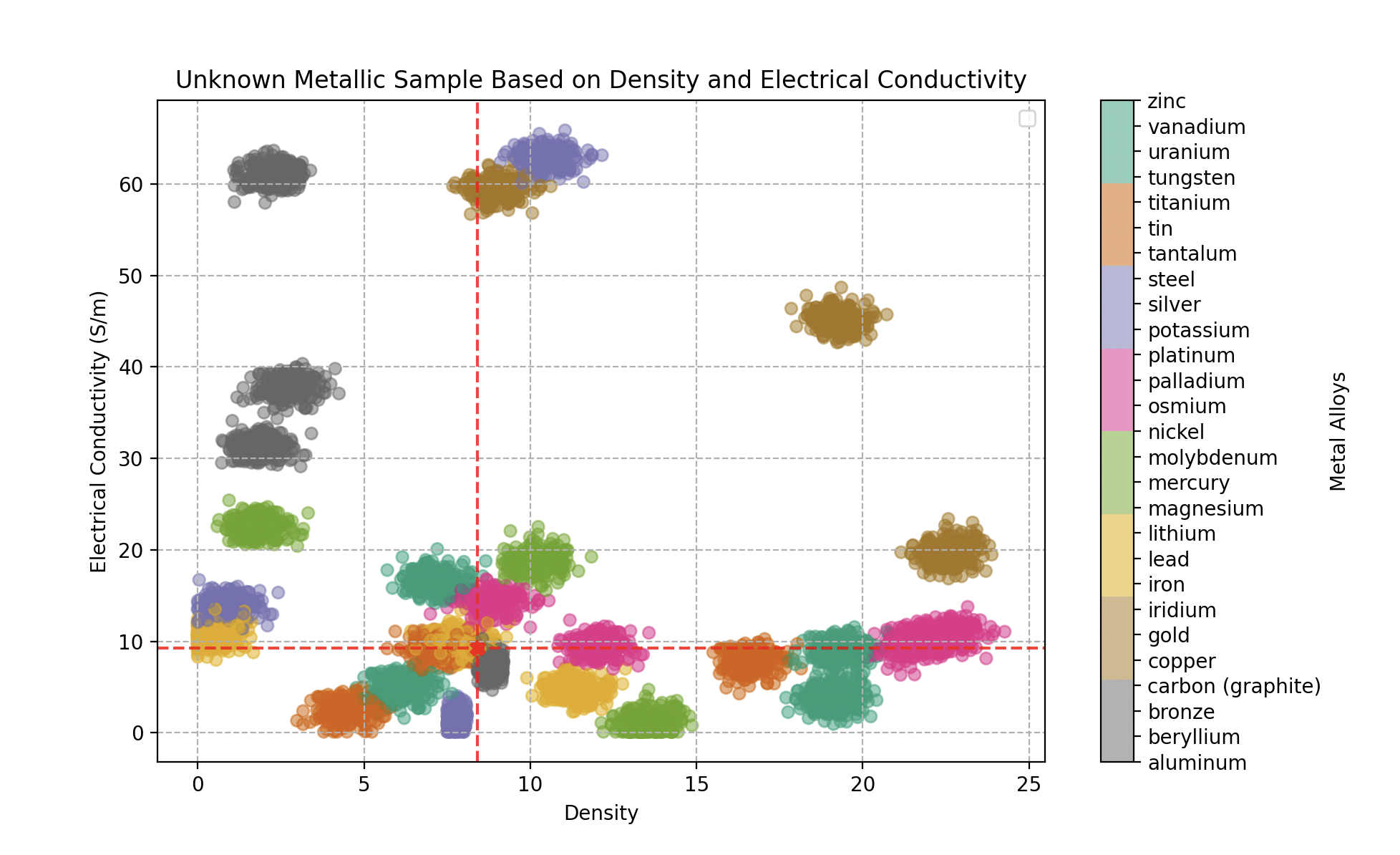
Classifying an unknown metallic sample: an iron alloy (70% iron, 20% bronze, 10% tin).

• The second (density 8.4, conductivity 9.26 GS/m): 70% iron, 20% bronze, 10% tin.

Classifying an unknown metallic sample: a vanadium alloy (70% vanadium, 25% tin, 5% iron).

• The third (density 7.5, conductivity 5.8 GS/m): 70% vanadium, 25% tin, 5% iron.

The Art of Model Selection

Train and Test

Wall-E quickly grasps the importance of never evaluating his model on the same data used for training. He splits the dataset into two parts:

• Train set (80%): dedicated to training the model.
• Test set (20%): held out for the final evaluation.

Credits: Disney/PIXAR

Model Validation

To tune hyperparameters (such as the number of KNN neighbors), Wall-E introduces a third section: the validation set. He compares different models — KNN with 2, 3, 20, or 100 neighbors — following this methodology:

1. Train the models on the training set.
2. Select the model with the best performance on the validation set.
3. Evaluate that chosen model on the test set.

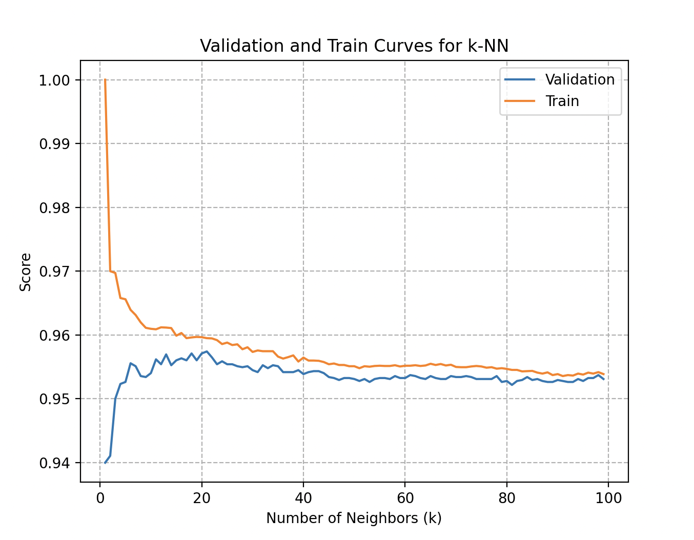
Validation and training curves: accuracy as a function of the number of neighbors used in the KNN algorithm.

More precisely, the validation curve for the number of neighbors $k$ in KNN answers key questions:

• Overfitting: a significant gap between training and validation scores indicates that the model is too complex and loses generalization.
• Underfitting: conversely, a model that has not learned the patterns in the training data shows poor performance and unreliable predictions.
• Parameter sensitivity: observing performance variations helps pick an optimal value of $k$.

In Wall-E’s case, both curves quickly reach 95.7% accuracy at around 20 to 25 neighbors.

Cross-Validation

Wall-E uses the K-fold method (with 5 partitions). During training, the model is systematically trained on $K-1$ partitions and validated on the remaining one, repeating this process $K$ times. He also exploits Stratified K-fold, which preserves the class distribution within each fold.

Learning Curves

Curious to know whether his model could benefit from additional data, Wall-E examines the learning curves. While adding data initially improves performance, those benefits eventually plateau.

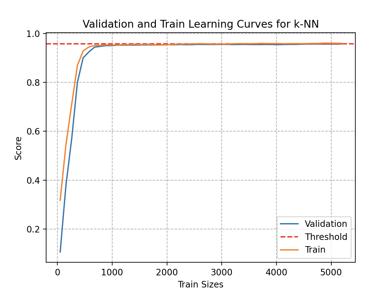
Examining this curve, he notices that a sufficiently accurate estimate could have been obtained with fewer than 1000 metal samples. Even accumulating 300 samples for each type (8100 objects total), accuracy plateaus at 95.7%.

The End of a Trilogy, the Beginning of a Technological Era

This last episode marks the conclusion of the captivating saga of the little robot Wall-E — an adventure that began with the foundations of machine learning. From his first steps in the realm of artificial intelligence, Wall-E has evolved through several chapters, exploring the basics of supervised learning, diving deep into regression, and finally climbing the complex peaks of classification.

This saga, rich in lessons, closes with the certainty that Wall-E is now ready to face new challenges in the complex world of artificial intelligence.

Credits: Disney/PIXAR

Bibliography

• G. James, D. Witten, T. Hastie and R. Tibshirani, An Introduction to Statistical Learning, Springer Verlag, 2013
• D. MacKay, Information Theory, Inference, and Learning Algorithms, Cambridge University Press, 2003
• T. Mitchell, Machine Learning, 1997
• C. Bishop, Pattern Recognition and Machine Learning, Springer, 2006
• J. Tolles, W-J. Meurer, “Logistic Regression Relating Patient Characteristics to Outcomes”, JAMA, 316 (5): 533–4, 2016
• B-V. Dasarathy, Nearest Neighbor (NN) Norms: NN Pattern Classification Techniques, 1991