
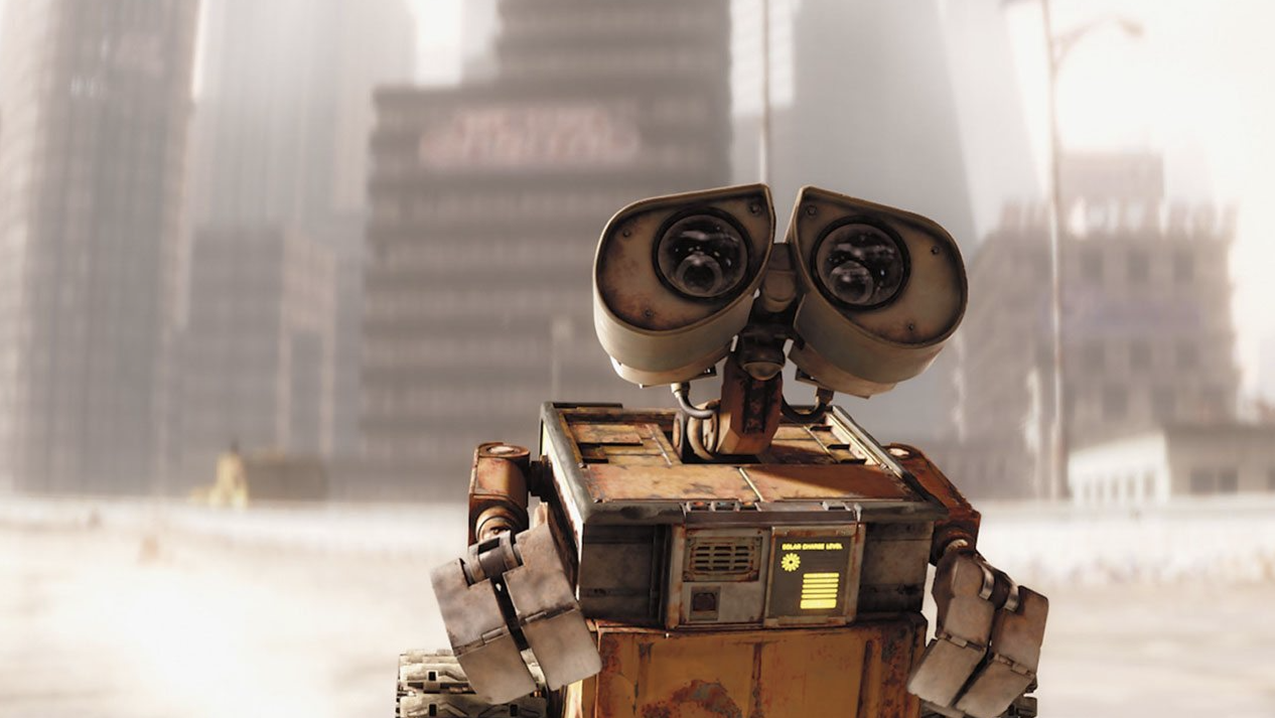
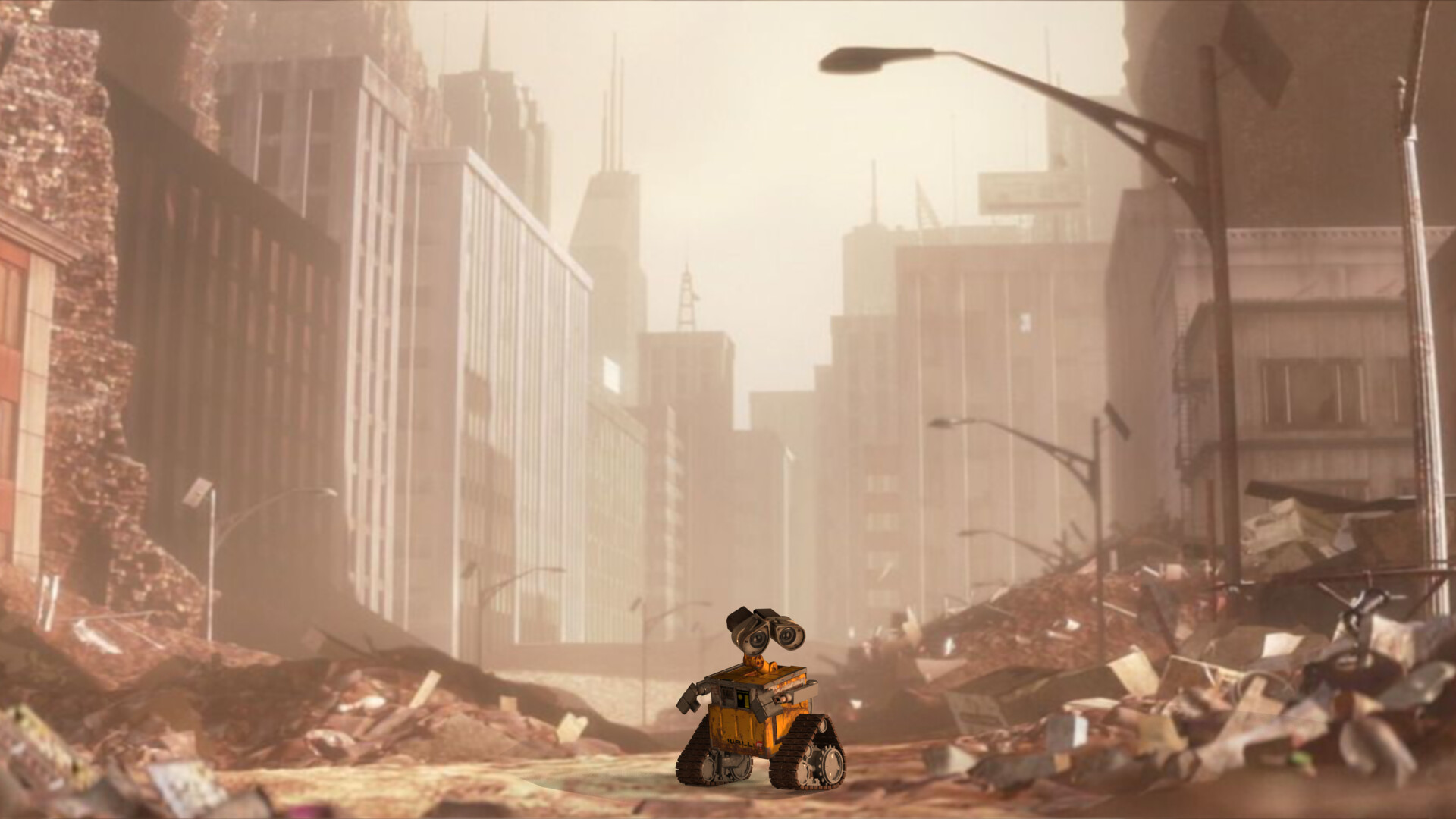
In a devastated post-apocalyptic world, where the remnants of human civilization are buried under massive heaps of waste, a solitary little robot named Wall-E navigates through this dystopian landscape. His mission: the methodical recycling of discarded waste that has accumulated over the years. However, Wall-E’s endeavors go beyond merely sorting pieces of plastic, metal sheets, and organic materials.
Through his interactions with the environment, this dedicated robot also gathers an abundance of information, analyzes millions of data points, and learns from his experiences to adapt, survive, and carry out his tasks with remarkable efficiency. The capabilities of what seemed to be a simple waste-collecting robot reveal the foundations of a burgeoning field: artificial intelligence.
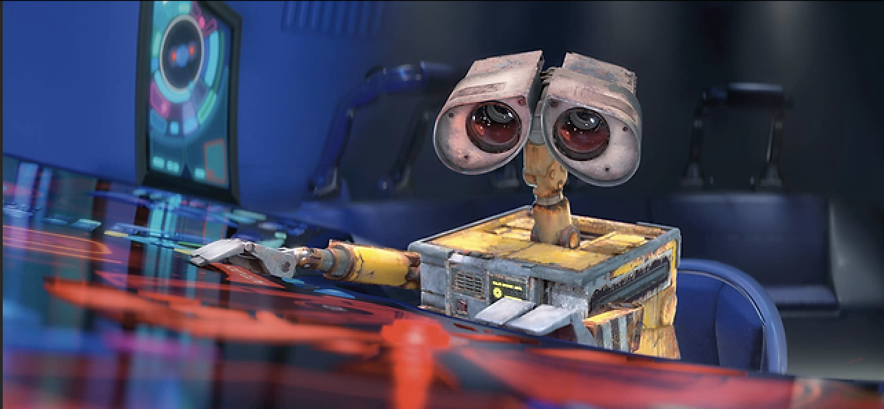
Credits: Disney/PIXAR
The Very Essence of Artificial Intelligence: Learning
In the early sparks of its existence, our little robot, much like a computer, was born to plunge into the abyss of calculations that would take millions of years for a human to find an answer to. Tasks once titanic for earthly souls stood before it, demanding to be tamed.
But within its circuits, a transformation was underway — inspired by the geniuses of the world’s scientific community. They infused our robot with a unique form of intelligence, a digital spark that changed the game. Wall-E, once a machine, was now becoming an entity that would learn and make complex decisions. It was the dawn of artificial intelligence, a new technological era.
Confronted with ever-growing challenges, Wall-E showcased its versatility. It seamlessly navigated both types of situations that humanity presented to it. In one case, it obediently followed calculations programmed by humans, responding like a calculator would to a simple .
Yet, it encountered a much more intricate puzzle: how to differentiate between the types of waste it encountered? How to recognize plastic from metal or organic material? Or more generally, how to solve a given problem without knowing the specific calculation required for its solution? This is where learning comes into play, a fascinating method we call Machine Learning. A method that opens a door when we don’t know which key to use. Machine learning is a master key for a multitude of tasks: image recognition, stock market predictions, estimating gold values, detecting cybersecurity vulnerabilities, and, of course, in our case: waste sorting.
To bestow this computer with learning intelligence, methods inspired by our own learning process were implemented. Among them, three fundamental approaches stand out.
Supervised learning forms the cornerstone of machine learning. Much like our own experience of acquiring knowledge, this method guides the little wheeled computer by providing it with pre-labeled examples. Like an eager apprentice, Wall-E is exposed to situations where the expected outcomes are already known. Then, by observing these examples, it gradually generalizes the relationships between inputs and outputs, enabling it to make decisions and solve similar problems it will encounter later on.

Credits: Disney/PIXAR
Unsupervised learning is a more open and exploratory form of artificial intelligence. This method allows the computer to autonomously discover hidden structures and patterns within data, without the need for pre-labeled examples. Like a fearless explorer, Wall-E uses its sensory analysis to discern patterns, group similar information, and explore the nuances of its environment.
Reinforcement learning relies on a system of rewards and punishments to guide the computer in its learning process. Similar to our own motivations, Wall-E is rewarded when it successfully accomplishes a task and faces negative consequences for failures. These encouragements and penalties enable it to optimize its actions, make intelligent decisions, and refine its skills over time.
Credits: Disney/PIXAR
Baby Robot Will Grow Up: the Architecture of Supervised Learning
At the birth of Wall-E, humanity had already charted its exodus to the distant corners of space, leaving behind an Earth suffocated under the weight of climate change and invasive pollution. The natural balances that had cradled our world for so long had faltered, relegating the planet to a new reality. Once vibrant cities teeming with life were now mere remnants, silent witnesses of a bygone era.
However, a group of scientists had committed to remain on this weary land, guided by a bold vision: to educate this small robot brimming with potential, to differentiate metals, to sort plastics — all for a crucial mission: to clean and regenerate the planet itself.
Credits: Disney/PIXAR
Thus began a phase of learning, where human knowledge was imparted to Wall-E. Scientists employed a specific method to guide this apprentice robot: supervised learning. This foundational aspect of machine learning provided Wall-E with the opportunity to evolve and grow by absorbing clearly labeled examples.
The beginnings of this journey revolve around four crucial elements: the dataset, the model and its parameters, the cost function, and the learning algorithm.
1. The Dataset: a Treasure Trove of Information
Like a gold mine for Wall-E, the dataset constitutes an organized collection of examples upon which the robot will base its learning. Each example consists of diverse input variables (features) arranged into a matrix, and corresponding expected outputs (targets) arranged into a vector. These final variables are what Wall-E will seek to predict.
For instance, if we wish to teach Wall-E to recognize types of waste, the specific characteristics of the objects will constitute the input data (density, electrical conductivity, carbon content, etc.), and labels indicating the type of each object will constitute the expected outputs (plastic, metal, organic).
| Index | Density | Electrical Conductivity () | Carbon Content | Material |
|---|---|---|---|---|
| 1 | 4.5 | 0 | Metal | |
| 2 | 0.5 | 0.5 | Organic | |
| 3 | 19.3 | 0 | Metal | |
| 4 | 1.1 | 0.4 | Organic | |
| 5 | 1.2 | 0 | Plastic |
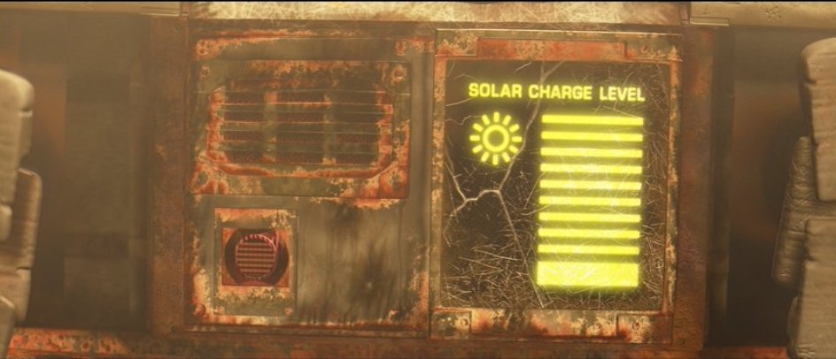
Of course, as a waste-sorting robot, this task constitutes its main mission. However, our little robot is also passionate about estimating the price of metals, especially gold. As it doesn’t truly grasp the human monetary system, it converts everything into bolts.
To entertain it, scientists have it analyze every piece of gold-like metal to determine its purity and assign it a market value. Here is an illustrative example with 5 samples.
| Index | Purity | Gold Price |
|---|---|---|
| 1 | 0.374540 | 1224.193388 |
| 2 | 0.950714 | 1483.925567 |
| 3 | 0.731994 | 1360.214557 |
| 4 | 0.598658 | 1284.274057 |
| 5 | 0.156019 | 1004.083221 |
With a much larger training dataset, Wall-E will be able to learn to classify metal, plastic, and organic materials based on their characteristics, and assess the price of an unknown metal based on its purity.
2. The Model and its Parameters: the Architecture of Learning
Now, let me introduce you to the structure that Wall-E will use to learn from the dataset. Imagine a “black box” — an electronic device that Wall-E uses to process information and make predictions. It is “black” in the sense that its internal workings are somewhat mysterious and complex, at least from Wall-E’s perspective. Inside this box, there are gears, levers, and hidden mechanisms that transform inputs (the data collected by Wall-E) into outputs (the predictions made by Wall-E).
Within this black box are the parameters. These are the internal settings that Wall-E can adjust to improve its ability to make accurate predictions — the secret buttons and knobs that Wall-E can turn and press to make the black box work more effectively. When we talk about a model, we are referring to a specific configuration of this black box.
Supervised learning consists of adjusting the parameters of this black box so that the predictions it generates are as close as possible to the correct answers (labels) provided in the training dataset. By adjusting the parameters and observing how predictions change, Wall-E tries to understand how this black box actually works and how to make it better.
These models can be of different natures: some are linear, others are non-linear.
Linear Models: Simplicity in Linearity
Linear models are relatively simple yet powerful mathematical representations. They assume that the relationship between inputs and outputs is linear — meaning it can be represented by a straight line (or a plane or hyperplane in a multidimensional space).
Scientists didn’t just limit the robot to simple waste recycling; they also taught it how to estimate the price of a metal based on its purity. By revisiting its data, Wall-E has a dataset consisting of samples of gold, where purity is the input feature and the corresponding price is the target .
| Index | ||
|---|---|---|
| 1 | 0.374540 | 1224.193388 |
| 2 | 0.950714 | 1483.925567 |
| 3 | 0.731994 | 1360.214557 |
| 4 | 0.598658 | 1284.274057 |
| 5 | 0.156019 | 1004.083221 |
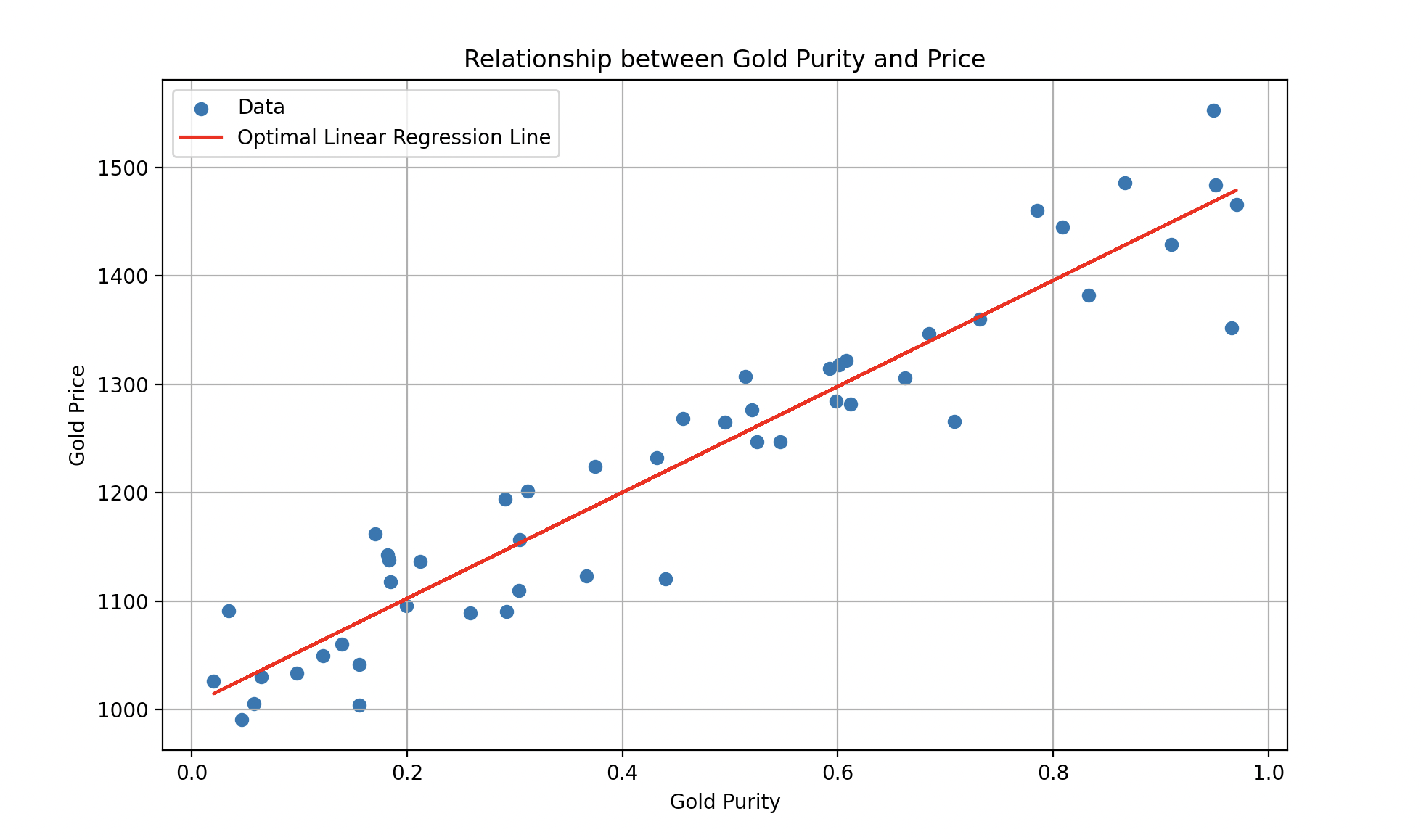
Sample 2, for instance, has purity and is worth bolts. Plotting the data (50 samples instead of 5, and imagining there could be millions):
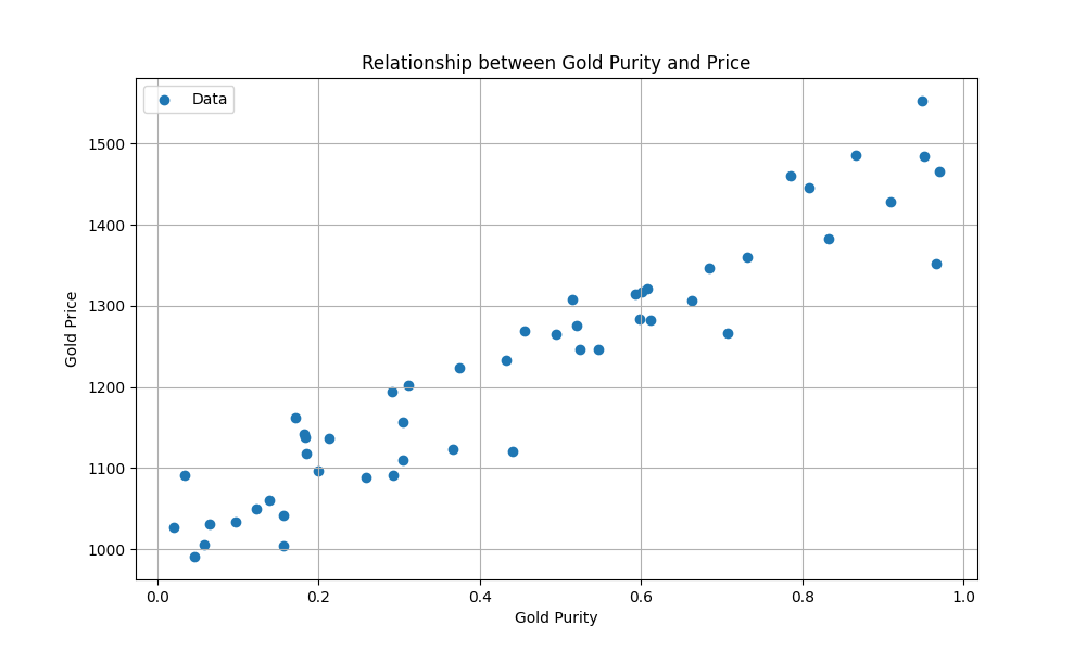
Credits: Disney/PIXAR — Scatter plot of gold price vs. purity.
Such a model could be represented by an equation of the form , where (the slope) and (the intercept) are adjustable parameters. Supervised learning aims to find the optimal values of and so that the model draws the best possible line that minimizes the error between predictions and actual values.
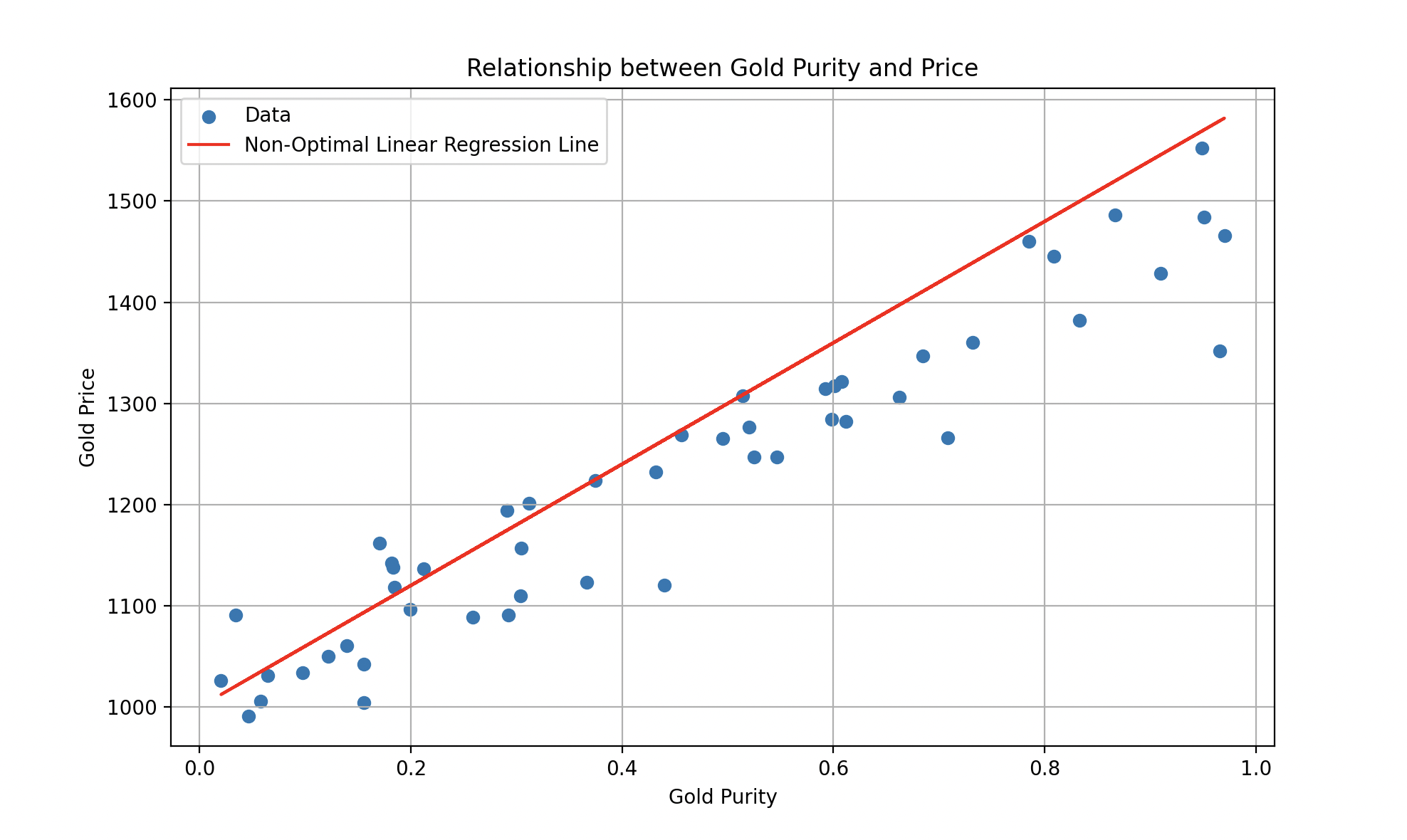
A fitted linear regression line on gold price as a function of purity.
Of course, reality is more complex than that, and for a more accurate estimation of the gold price, it would be necessary to consider historical information about gold prices over time, as well as relevant economic, political, and geopolitical features. While linear models are simple and easy to interpret, they can be limited in their ability to capture complex relationships between variables. This is where non-linear models come into play.
Non-linear Models: Elegance in Complexity
Non-linear models offer increased flexibility compared to linear models. They are capable of capturing complex relationships between inputs and outputs, allowing the representation of more sophisticated data behaviors. Imagine that we have data behaving more like this:
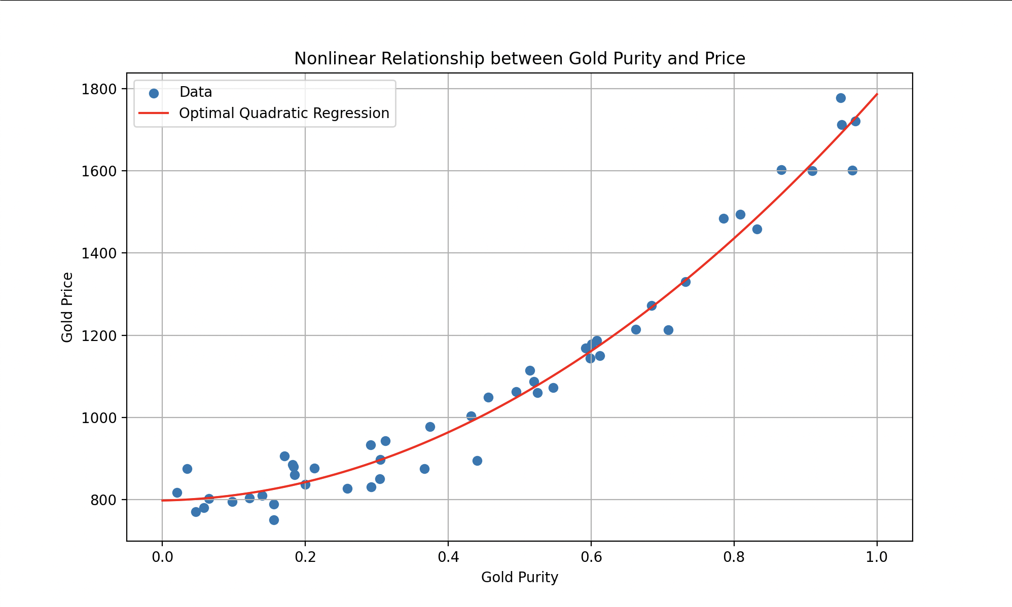
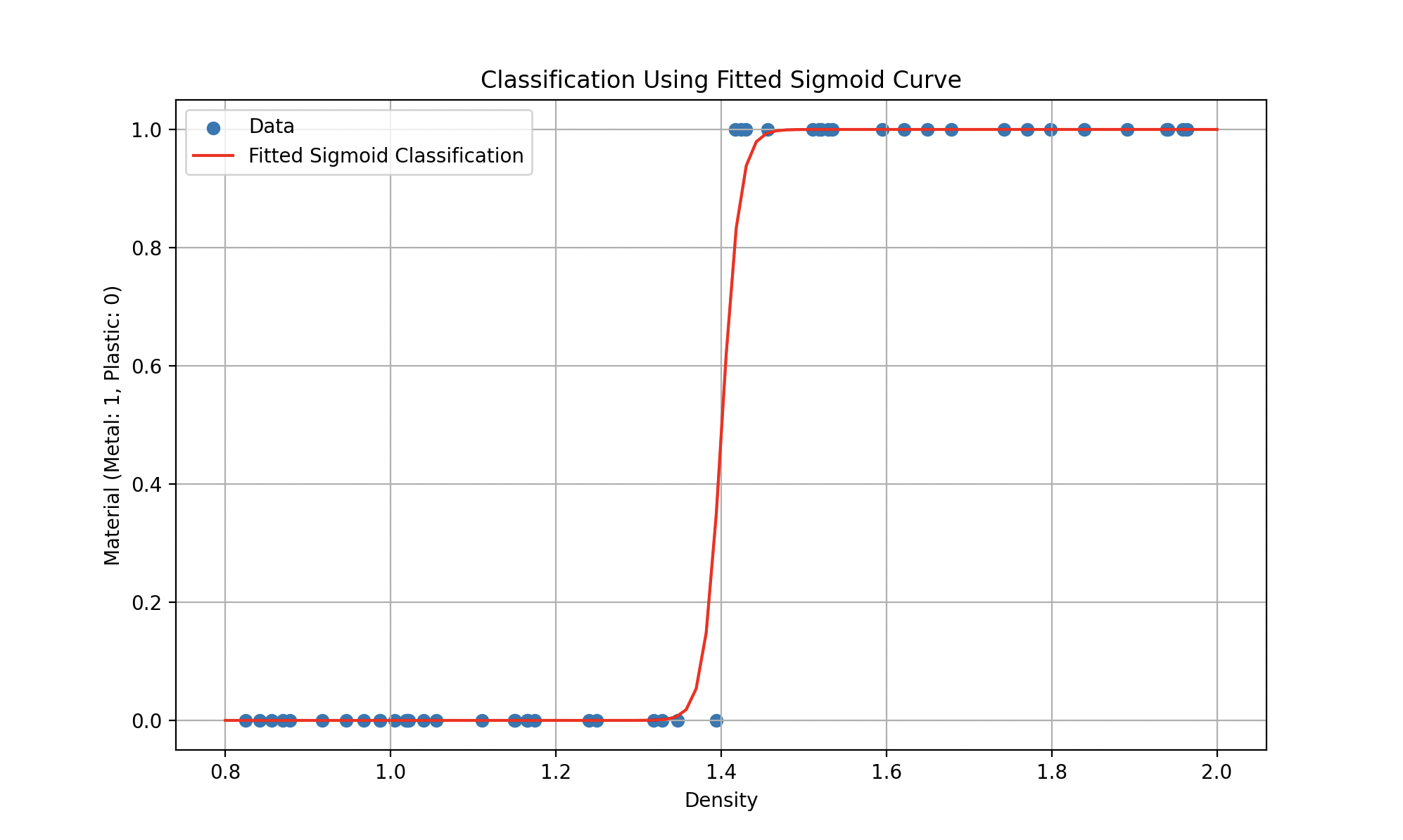
Left: gold price estimation with a polynomial. Right: plastic vs. metal classification with a sigmoid.
Such models could be represented by equations like (a quadratic polynomial for the first curve) or more complex functions (like the sigmoid for the second), where the goal remains to find the parameters that minimize the error.
Credits: Disney/PIXAR
The choice between a linear and a non-linear model depends on the nature of the data and the complexity of the problem. Linear models are generally preferred when relationships are simple and clear, while non-linear models are favored for more complex tasks.
3. Cost Function: Measuring Errors
To measure how well Wall-E performs in this gold estimation task, we use a special function called the cost function. This function plays a crucial role in quantifying the errors between the price estimates made by Wall-E and the actual gold prices from historical data. It calculates the error for each estimate and then sums up these errors to form an overall measure of Wall-E’s performance.
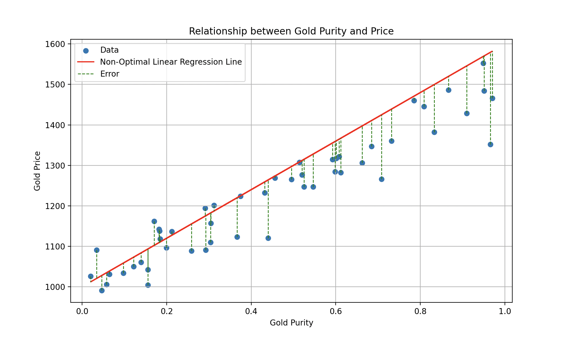
The vertical green segments represent individual errors between the predicted line and each data point.
Being a true perfectionist, Wall-E aims for a cost function as small as possible. Minimizing it means minimizing the errors between his price estimates and the actual prices, in order to make predictions with the highest possible accuracy.
4. The Learning Algorithm: Finding the Optimum
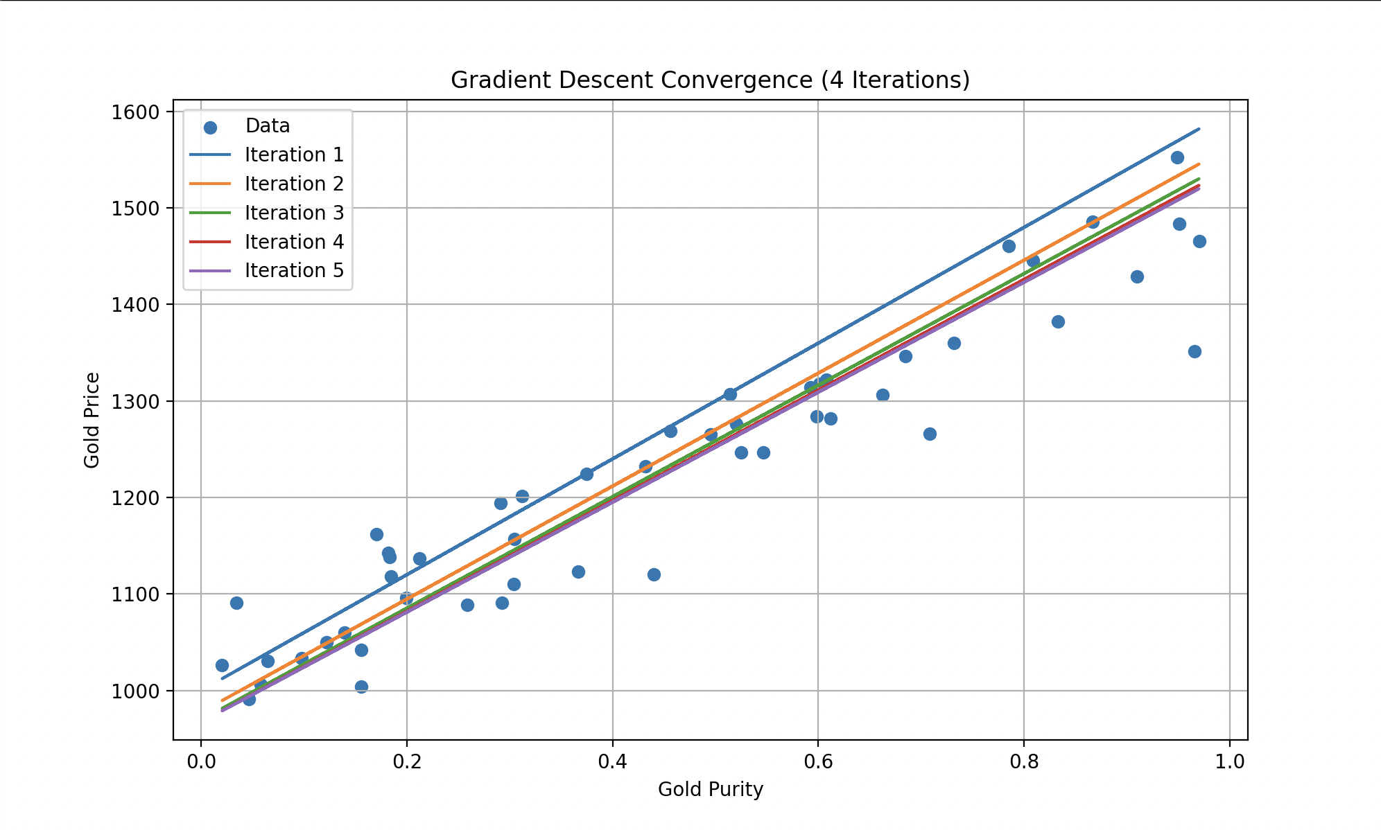
To reduce this cost function, Wall-E employs a well-known algorithm called gradient descent. This technique enables it to gradually adjust its internal parameters (for the linear model: and ) based on the errors made during the gold price estimation. At each step of the learning process, Wall-E enhances its performance by moving closer to the optimum, where the cost function is minimized.
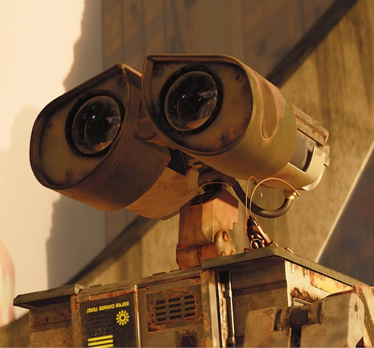
Left: cost history along iterations. Right: Wall-E doing the math (Disney/PIXAR).
We observe that with each iteration, the errors become progressively smaller until they reach a constant level. Wall-E becomes an expert in gold price estimation, making predictions with remarkable accuracy.
Final fitted curve. A gold sample with purity 0.8 would be priced around 1400 bolts.
A Super Robot
Wall-E’s learning universe extends across many applications, falling into two distinct families: regression and classification.
Regression is a quantitative technique used to predict continuous target values — numbers that can take any value within a certain range. Estimating the price of gold falls under regression. Other examples Wall-E could tackle:

Credits: Disney/PIXAR
- Estimation of remaining drinkable water: combining historical data on groundwater levels, precipitation, and evaporation rates to estimate underground reserves and help humans plan their use of this vital resource.
- Prediction of solar energy production: using daily sunlight, panel quality, and weather data to forecast solar output across the day and across conditions.
Credits: Disney/PIXAR
- Battery lifespan estimation: analyzing past battery performance and environmental conditions to predict remaining lifespan and plan proactive replacements.
- Prediction of pollution levels: gathering data on air and water pollution, plus dumping practices, to predict future pollution and identify the most critical areas for sanitation.
Classification is another supervised-learning technique used to predict discrete labels or categories. In its quest to clean up the Earth, Wall-E must sort waste of every kind. Using data on shape, size, composition, and hazardousness, it can build a classification model to assign objects to classes (plastic, metal, organic, toxic, etc.). A few applications:

Credits: Disney/PIXAR
- Classification of celestial objects: identifying asteroids, comets, planets, and other bodies based on their characteristics and trajectories.
- Classification of human emotions: gathering facial expressions, gestures, and vocal tones to recognize joy, sadness, fear, or anger — and adapt interactions accordingly.
Credits: Disney/PIXAR
- Classification of extraterrestrial signals: detecting and distinguishing greeting messages, mathematical patterns, or warnings as Wall-E scans the stars.
Exploration and Enrichment
As it evolved in this intricate world, the little solitary robot demonstrated unmatched mastery with every challenge it faced. Its journey started humbly as a mere waste collector, but it evolved to become an expert in value estimation — uncovering the profound foundations of artificial intelligence. Supervised learning, the cornerstone of this intelligence, allowed Wall-E to transcend the limitations of its machine nature and become an agile learner.
The upcoming sections delve into two crucial aspects of supervised learning in more detail.
Part II — The Little Gold Miner: the regression model that enabled Wall-E to gain an in-depth understanding of gold value estimation. From dataset analysis to model design, employing the cost function and the gradient descent algorithm, each step is methodically dissected.
Part III — Waste Allocation Load Lifter: Earth Class: the realm of waste sorting, a task both critical and challenging. We detail how Wall-E used classification models to learn to distinguish different types of waste — from binary plastic-vs-metal sorting to multi-class metal identification with KNN.
Just as Wall-E learned to differentiate plastic from metal and estimate gold purity, artificial intelligence finds its place in domains ranging from predicting solar energy production to classifying human emotions. The path Wall-E has treaded is only a prologue.
Bibliography
- G. James, D. Witten, T. Hastie and R. Tibshirani, An Introduction to Statistical Learning, Springer Verlag, coll. “Springer Texts in Statistics”, 2013
- D. MacKay, Information Theory, Inference, and Learning Algorithms, Cambridge University Press, 2003
- T. Mitchell, Machine Learning, 1997
- F. Galton, Kinship and Correlation (reprinted 1989), Statistical Science, vol. 4, no. 2, pp. 80–86
- C. Bishop, Pattern Recognition and Machine Learning, Springer, 2006